
Advanced Retrieval: Long Context, Contextual Retrieval and Late Chunking
Long context vs RAG, contextual retrieval and late chunking: fix what each chunk means.
Everything up to here has been about making a conventional pipeline work: split well, embed consistently, retrieve broadly, rerank, observe, cache, ship. This part is where the course turns to the 2026 frontier, and it opens by attacking the premise of the whole guide.
Three techniques, three different boxes of the mental model:
- Long context asks whether Phase A (index) needs to exist at all. If the model can
read a million tokens, why split, embed and store anything? The answer is arithmetic, not ideology.
- Contextual retrieval modifies the
[Contextualize]step in Phase A — the one box in
the diagram that has been empty until now. It changes the text you embed.
- Late chunking modifies the
Split → Embedordering in Phase A. It changes **when the
embedding is computed**.
All three are governed by invariant 3: index-time cost is one-time and amortized; query-time cost recurs on every request. Contextual retrieval and late chunking are pure plays on that invariant — they spend heavily on the write path and nothing on the read path. Long context is the opposite bet: skip the write path entirely and pay forever on the read path. That is the entire argument of this part in three sentences.
The code lives in the second repo, fcc-production-rag-part-6 (the "Advanced RAG 2026" lessons 6.1–6.3): 01_long_context_vs_rag.py, 02_contextual_retrieval.py, 03_late_chunking.py. Chapters 24, 25 and 26 of the source cover them at 06:06:09 → 06:42:04. Three rows of the repo README's six-row Part 6 table belong to this part:
| Technique | What it solves | Claimed improvement |
|---|---|---|
| Long Context vs RAG | When to use 1M token windows vs retrieval | Cost optimization |
| Contextual Retrieval | Chunks losing document context | 67% fewer retrieval failures |
| Late Chunking | Cross-chunk context lost in embeddings | 10–12% accuracy boost |
Hold those two percentages lightly. By the end of this part you will know where each one comes from, which configuration it actually measures, and why the course's own instructor tells you twice to ignore them and measure your own.
1. Is RAG dead? The long-context question
1.1 The question, and the reframe
06:06:15 The chapter opens mid-sentence on the single most common question the instructor receives: with models like Gemini shipping million-token windows, do we still need RAG? His answer is a refusal to answer the question as asked, repeated three times in eight minutes:
"Don't disregard one over the other. Just figure out when to use which." 06:11:20
The script itself prints the reframe as a banner before it does anything else:
# fcc-production-rag-part-6/01_long_context_vs_rag.py — __main__ banner
print("\nThe question isn't 'Is RAG dead?'")
print("It's 'When should I use RAG vs Long Context?'")
Define terms precisely, because the comparison is meaningless otherwise. Long context, as used here, means stuffing the entire corpus into the prompt window on every query, with no retrieval step at all — no splitter, no embeddings, no vector store. RAG means retrieving four to eight chunks (~2K tokens) and sending only those. This is a comparison of two architectures, not of two models.
1.2 The comparison table as spoken
| Dimension | RAG | Long context |
|---|---|---|
| Cost per query | no number spoken — "very insignificant per query" | ~$0.10 |
| Latency | ~1 second | ~45 seconds |
| Scaling | "unlimited, really" | ~1M token limit |
| Headline | "RAG is over 1,200 times cheaper" 06:06:15 | — |
There is no screenshot for chapter 24 — INDEX.md lists it explicitly under "chapters with no screenshot" — so every figure above comes from the auto-generated transcript, and the RAG cost cell is never read aloud at all. That single number is simply lost. The 1 s vs 45 s pair and the 1,200× ratio are transcript-derived and uncited; treat them as directional.
"It's the difference between having a viable product and bankruptcy." 06:07:16
1.3 The cost arithmetic, and why it prints 25× and not 1,200×
calculate_costs() is pure arithmetic. It makes no API call. That matters: you can run it, change its constants and reason about your own numbers without spending a cent.
# fcc-production-rag-part-6/01_long_context_vs_rag.py — calculate_costs(), abridged:
# the print() calls that only echo these values are omitted.
# Docstring pricing: GPT-4o (April 2026) — input $2.50 / 1M, output $10.00 / 1M.

# Scenario: Query against 100K tokens of documentation
doc_tokens = 100_000
query_tokens = 100
output_tokens = 500

# Long Context approach - stuff everything
long_context_input = doc_tokens + query_tokens
long_context_cost = (long_context_input * 2.50 / 1_000_000) + (
    output_tokens * 10.00 / 1_000_000
)

# RAG approach - retrieve 4 chunks of ~500 tokens each
rag_chunks = 4
tokens_per_chunk = 500
rag_input = (rag_chunks * tokens_per_chunk) + query_tokens
rag_cost = (rag_input * 2.50 / 1_000_000) + (output_tokens * 10.00 / 1_000_000)

print(f"RAG is {long_context_cost / rag_cost:.0f}x cheaper per query!")

queries_per_day = 10_000
print(
    f"  Monthly savings with RAG: ${(long_context_cost - rag_cost) * queries_per_day * 30:.2f}"
)
Work it out by hand, because the arithmetic is the lesson:
| Quantity | Long context | RAG (4 × 500) |
|---|---|---|
| Input tokens | 100,100 | 2,100 |
| Input cost @ $2.50/1M | $0.25025 | $0.00525 |
| Output cost (500 tok @ $10/1M) | $0.00500 | $0.00500 |
| Cost per query | $0.25525 | $0.01025 |
| At 10,000 queries/day | $2,552.50/day | $102.50/day |
| Monthly delta (×30) | — | $73,500.00 saved |
06:11:20 He reads the printed line off the screen: "RAG is 25x cheaper per query" (0.25525 / 0.01025 = 24.9, formatted :.0f). But the slide he showed five minutes earlier said over 1,200×. Both numbers are stated in the same eight minutes and never reconciled.
Two more traps in this function that a reader will hit within a minute of running it:
1.4 The latency demo, and why you should not quote it
compare_latency() is the only function in the file that makes real API calls. It times two llm.invoke() calls, one with a one-sentence context and one with the same sentence repeated 50 times.
# fcc-production-rag-part-6/01_long_context_vs_rag.py — compare_latency()
small_context = (
    "The company's return policy allows returns within 30 days with receipt."
)
large_context = (small_context + "\n\n") * 50  # ~2500 tokens

query = "What is the return policy?"

start = time.time()
response_small = llm.invoke(f"Context: {small_context}\n\nQuestion: {query}")
small_time = time.time() - start

start = time.time()
response_large = llm.invoke(f"Context: {large_context}\n\nQuestion: {query}")
large_time = time.time() - start

print(f"\nSmall context (~50 tokens): {small_time:.2f}s")
print(f"Large context (~2500 tokens): {large_time:.2f}s")
print(
    f"Difference: {large_time - small_time:.2f}s ({large_time/small_time:.1f}x slower)"
)
print("\nNote: At 100K+ tokens, latency difference is much more dramatic!")
The live run 06:12:23 produced 1.45 s small and 1.16 s large — a difference of −0.29 s and a printed "0.8x slower". The demo's own numbers say long context was faster.
1.5 The reliability ceiling: a 1M window is not 1M usable tokens
06:07:16 The most important non-monetary claim in the chapter:
"these models become unreliable around 60 to 70% of that limit." 06:07:16
Effective, reliable capacity is roughly 60–70% of the advertised window — about 600K–700K tokens on a 1M-token model. Past that, in-context retrieval degrades: the "lost in the middle" / context-rot family of failures, where the model demonstrably stops attending to material it was given. His framing: "this is not just about money or economics" — even with an infinite budget, the accuracy story alone argues against naive stuffing.
He asserts this as "a known fact" and names no paper and no benchmark. It is consistent with the published long-context literature, but as delivered in this course it is an uncited claim. Treat 60–70% as a planning heuristic, not a spec: a million-token window buys you 600–700K tokens of trustworthy attention, so budget against the effective limit, not the marketing limit.
The spoken lists — where each approach genuinely wins
Before the printed framework, he narrates two informal lists. They differ from the script's printed box in places and both are worth having.
Where long context genuinely wins 06:07:16 — "now let's be fair, there are cases when long context models are really good":
- Small document size — smaller documents overall.
- Under 100K tokens — *"if you have less than 100k tokens that will be a good way of
dealing with this"*. (The printed box says <50K. Both numbers are in the lesson.)
- Static, bounded tasks — a task whose input does not grow and whose scope is fixed.
- You need the entire context simultaneously — whole-document reasoning where any chunk
boundary would destroy the answer: summarise this contract, find contradictions across the whole document.
Where RAG wins 06:08:17:
- Large knowledge base — *"a lot of documents, a lot of information that you're putting
in a vector database"*.
- Dynamic, frequently updated content — "RAG is really good at that". (Contradicts the
printed box; see the callout below.)
- Cost effectiveness — "if your system is cost sensitive, then RAG is the way to go".
- Precision — *"if you want to have a system that is very precise and very specific then
RAG definitely wins the race" — with the crucial conditional "if all things are put together correctly"*.
1.6 The decision framework
print_decision_framework() prints an ASCII box — it is a print statement in the script, not a slide — and it is the reusable artefact of the whole chapter. Reproduced faithfully, with the spoken variants noted:
| Use long context when | Use RAG when |
|---|---|
| Corpus is small (<50K tokens) — he says <100K aloud at 06:07:16 | Corpus is large (>100K tokens) |
| Query volume is low (<100 queries/day) | Query volume is high (1000s/day) — he says "hundreds" aloud 06:13:23 |
| You need to analyse the ENTIRE document | Users ask about specific topics, not whole-doc analysis |
| Documents change frequently (no embedding overhead) | Documents are relatively stable |
| Simplicity > cost optimization | Cost and latency matter |
| — | You need citations / source tracking |
Embedding overhead, defined: the cost, latency and operational burden of embedding and indexing every document version into the vector store — and re-doing it whenever a document changes. It is the one thing long context lets you skip entirely.
Two more asymmetries worth stating plainly, because the printed box only implies them:
- Citations are structurally free in RAG and structurally hard in long context. In RAG
you know which chunk produced the answer because you put it there. Stuff 100K tokens in one blob and attribution becomes a second, unreliable LLM task.
- RAG's precision is conditional. *"RAG provides lots of precision **if all things are
put together correctly**"* 06:08:17. That conditional clause is Parts 3 through 9 of this guide. RAG does not win on precision by default; it wins on precision when its pipeline is built right.
1.7 The hybrid approach: RAG selects, long context reads
The synthesis, delivered at the chapter boundary 06:14:29:
"Don't separate the two — RAG versus long context. You say RAG AND long context."
And the line he closes on: "All in all, RAG is not dead." The mechanism is two steps and it is the shape most real systems should converge on:
- RAG retrieves candidate documents — not chunks to answer from, documents to read.
- Load those full documents into the context window for the detailed answer.
The query shape that needs both: "tell me about X, Y and Z, and then analyse deeply this part of the corpus." RAG narrows the corpus from ten thousand documents to one; long context then does the careful reading on what survived.
demo_hybrid_approach() is the fourth call in __main__, so it does execute — but the narration stops after the decision framework and never discusses it, so this is the only place a reader will see it explained. The load-bearing detail is k=1:
# fcc-production-rag-part-6/01_long_context_vs_rag.py — demo_hybrid_approach()
# Step 1: Create vector store for RAG retrieval
embeddings = OpenAIEmbeddings(model="text-embedding-3-small")
vectorstore = Chroma.from_documents(
    documents=documents, embedding=embeddings, collection_name="hybrid_demo"
)

query = "What's the policy on working from home and what equipment do I get?"

# Step 3: RAG retrieves relevant document
retriever = vectorstore.as_retriever(search_kwargs={"k": 1})
relevant_docs = retriever.invoke(query)
print(f"Retrieved: {relevant_docs[0].metadata['source']}")

# Step 4: Load FULL document into context (hybrid part)
full_doc = relevant_docs[0].page_content

prompt = ChatPromptTemplate.from_messages(
    [
        (
            "system",
            """You are a helpful HR assistant. Use the full policy document
        below to give a comprehensive answer. Include all relevant details from
        the document.

        Policy Document:
        {document}""",
        ),
        ("human", "{query}"),
    ]
)

chain = prompt | llm
response = chain.invoke({"document": full_doc, "query": query})

# Cleanup
vectorstore.delete_collection()
k=1 is doing something unusual and deliberate: retrieval here picks the document, not the answer. The three demo documents are written as whole policies with Sections 1–4 (remote_work_policy.pdf, expense_policy.pdf, pto_policy.pdf), all tagged doc_type: "policy", so "load the full document" is a meaningful act. The query — *working from home and what equipment do I get* — deliberately spans Section 2 and Section 3 of one document, which is exactly the question a top-k chunk retrieval answers badly and a whole-document read answers perfectly.
The synthetic HR corpus, in case you want to reproduce the run
These are fixture values, not RAG parameters — but reproduce them exactly if you want the same retrieval behaviour.
- Remote Work Policy — eligibility after a 90-day probation (part-time case by
case); remote up to 3 days/week; core hours 10am–3pm local; laptop + monitor provided, employee pays for internet, $500 annual home-office stipend; reachable on Slack during core hours, video on in team meetings, 30-minute response expectation.
- Expense Reimbursement Policy — expenses over $500 need manager pre-approval,
travel over $2,000 needs VP approval; receipts required over $25 (digital accepted, card statements alone are not); submit within 30 days, late needs director approval; reimbursed within 10 business days by direct deposit.
- PTO and Leave Policy — 15 days PTO/year, +1 day per year of service up to
25; 10 days sick leave, no roll-over, doctor's note over 3 days; 10 paid holidays; unpaid leave up to 12 weeks for family/medical, FMLA rules apply.
Note vectorstore.delete_collection() at the end. Every demo in this part tears down its Chroma collection, and it is a habit worth copying: these scripts hard-code collection_names, and a crash mid-run leaves a populated collection behind that the next run appends to, silently corrupting the comparison.
The printed benefits: 1. RAG finds the RIGHT document quickly. 2. Full document context ensures nothing is missed. 3. Still cheaper than stuffing ALL documents. 4. Best for: "Find relevant doc, then analyze thoroughly."
1.8 The lesson underneath: think at scale, not at prototype size
06:12:23 is the paragraph he says is "exactly what I want to show you": when you start building RAG, the data volumes are tiny and every number looks trivially small, so you never notice the architecture you are committing to.
"So always think in scaling, not in small numbers." 06:12:23
It applies twice in this chapter and both applications are worth internalising:
- Cost. $0.255 vs $0.010 per query looks like nothing. Multiply by 10,000 queries/day
and 30 days and it is $73,500/month of avoidable spend.
- Latency. A 2,500-token demo shows no difference at all (even a negative one). At 100K+
tokens it becomes the 1 s vs 45 s of the opening table.
Key takeaways, as printed by the script:
- RAG is NOT dead — it's about cost and latency at scale.
- Long context wins for small docs, low volume, whole-doc analysis.
- RAG wins for large corpora, high volume, specific queries.
- Hybrid approach: RAG to find docs, long context to analyze.
- The future is using BOTH strategically.
2. Contextual retrieval: fix the chunk before you embed it
2.1 The disease
Part 3 established that chunking is architecture. This is the sequel: even a correctly split chunk can be unretrievable, because splitting severs a chunk from the document that made it meaningful.
"when you chunk, each one of these chunks loses its context." 06:15:33
His canonical example: a chunk that reads "the company policy states…" — which company? which policy? The file's docstring states it as "The company was founded in 1994" — Which company? What document is this from? The chunk is factually true and completely unattributable.
The failure is mechanical, not mysterious. 06:20:42 A user asks "What is ACME's revenue?" The chunk holding the answer reads:
"Revenue for fiscal year 2025 reached $4.2 billion, representing a 15% increase from the previous year."
The token ACME never appears. Neither lexical matching nor semantic matching has anything to hook onto. Pronouns and definite descriptions — "the company", "they", "it" — are the general form of this bug, and they are everywhere in real corpora: annual reports, policy manuals, technical documentation, anything with a title that the body text never repeats.
demonstrate_context_loss() prints the disease with zero API calls: an ACME Corporation Annual Report 2025 with three sections (Company Overview / Financial Highlights / Future Outlook), reduced to three deliberately orphaned chunks:
- "The company specializes in manufacturing industrial equipment for the mining sector."
→ which company?
- *"Revenue for fiscal year 2025 reached $4.2 billion, representing a 15% increase from the
previous year."* → for what company?
- "The company plans to expand into renewable energy equipment in 2026." → plans of what
company?
The two demo documents, in full — reproduce these to get the same numbers
Document 1 — the ACME Corporation Annual Report 2025 (used by demonstrate_context_loss(), demonstrate_contextual_retrieval() and compare_retrieval()):
ACME Corporation Annual Report 2025

Company Overview:
ACME Corporation was founded in 1994 in San Francisco. The company
specializes in manufacturing industrial equipment for the mining sector.

Financial Highlights:
Revenue for fiscal year 2025 reached $4.2 billion, representing a 15%
increase from the previous year. The company's profit margin improved
to 18%, up from 14% in 2024.

Future Outlook:
The company plans to expand into renewable energy equipment in 2026.
A new manufacturing facility will open in Austin, Texas. The company
expects revenue growth of 20% in the coming fiscal year.
(The transcript's "revenue for fiscal year 2005" is a mis-hearing of 2025.)
Document 2 — the TechStartup Inc. Series B press release (used by demo_production_pipeline(), metadata={"title": "TechStartup Inc. Series B Announcement", "source": "press_release.pdf"}): a Seattle-based AI infrastructure company closes a $45 million Series B led by Sequoia Capital with participation from Andreessen Horowitz; CEO Jane Smith expects to double headcount by end of 2026; flagship product AIFlow helps enterprises deploy and manage LLMs in production and serves 200+ enterprise customers.
Note how both documents were written: the entity name appears once, in the first paragraph, and every subsequent sentence says "the company". That is not a contrivance — it is how annual reports, press releases and policy manuals are actually written.
2.2 The mechanism, and the two words that matter
Contextual retrieval was published by Anthropic in late 2024 06:17:36. The technique is one sentence long:
"use an LLM to prepend context to each one of these chunks before embedding. The key word here is before embedding." 06:16:35
That is the whole load-bearing detail of the lesson. The added context is:
- generated by an LLM, not templated from metadata — the model reads the whole document
and writes a situating sentence;
- concatenated onto the chunk text prior to the embedding call, so the vector itself
encodes the document-level facts.
What the prefix carries: document-level information (title, report name, year, organisation) and section-level information (which part of the document this chunk sits in), plus resolution of whatever entities the chunk's pronouns point at. The retrievable unit now answers "which company?" by itself.
2.3 The core function, in full
This is the entire technique. It is one prompt template and an LCEL two-node chain — there is no bespoke subsystem here.
# fcc-production-rag-part-6/02_contextual_retrieval.py — add_contextual_prefix()
def add_contextual_prefix(
    chunk: str, full_document: str, document_title: str, llm: ChatOpenAI
) -> str:
    """
    Use LLM to generate a contextual prefix for a chunk.

    This is the core of Contextual Retrieval:
    - Give the LLM the full document and the specific chunk
    - Ask it to write a brief context that situates the chunk
    - Prepend this context to the chunk before embedding
    """

    prompt = ChatPromptTemplate.from_messages(
        [
            (
                "system",
                """You are an expert at adding context to document chunks.

Given a document and a specific chunk from that document, write a SHORT
context (1-2 sentences) that helps situate the chunk within the document.

The context should include:
- The document title/source if relevant
- Key entities mentioned earlier in the document
- Any important context that helps understand this chunk

Keep it brief - just enough to disambiguate the chunk.
Output ONLY the contextual prefix, nothing else.""",
            ),
            (
                "human",
                """Document Title: {title}

Full Document:
{document}

Chunk to contextualize:
{chunk}

Write a brief contextual prefix for this chunk:""",
            ),
        ]
    )

    chain = prompt | llm
    response = chain.invoke(
        {"title": document_title, "document": full_document, "chunk": chunk}
    )

    return response.content
Three things in that prompt are load-bearing and worth stealing verbatim:
- "1-2 sentences" and "Keep it brief" — the prefix inflates every chunk, so its
length is a cost you pay forever (see §2.7).
- "Key entities mentioned earlier in the document" — this is the instruction that
performs coreference resolution. It is why "the company" becomes "ACME Corporation".
- "Output ONLY the contextual prefix, nothing else." — without it, a chatty model
returns "Sure! Here's a context for that chunk:" and that preamble gets embedded as noise, permanently, into your index.
Both ChatOpenAI instances in the file use model="gpt-4o-mini", temperature=0. Determinism matters here: context generation is an extraction task, not a creative one, and temperature=0 means re-indexing the same corpus produces near-identical prefixes rather than a new set of vectors every time.
And the one line that is the technique — it appears twice in the file, once in the demo (line 201, as contextualized) and once in the production function (line 330, as contextualized_content):
# fcc-production-rag-part-6/02_contextual_retrieval.py:201
contextualized = f"{context_prefix} {chunk}"
The original sentence is never rewritten or destroyed. The prefix is purely additive — which is what makes the whole thing auditable.
Running it on the ACME chunks produces prefixes like 06:20:42:
- Chunk 1 → *"In the Company Overview section of the ACME Corporation Annual Report 2025,
the document introduces ACME…"* + original text
- Chunk 2 → "…Financial Highlights section of the ACME Corporation…" + original text
- Chunk 3 → "In the Future Outlook section of ACME Corporation Annual Report…" + original
text
2.4 The production function
create_contextual_chunks() is the drop-in replacement for your splitter step. It is what you actually ship.
# fcc-production-rag-part-6/02_contextual_retrieval.py — create_contextual_chunks()
def create_contextual_chunks(
    documents: list[Document],
    llm: ChatOpenAI,
    chunk_size: int = 500,
    chunk_overlap: int = 100,
) -> list[Document]:
    """
    Production-ready function to create contextualized chunks.

    This is the function you'd use in a real RAG pipeline.
    Note: This adds latency and cost during indexing, but it's a one-time cost.
    """

    text_splitter = RecursiveCharacterTextSplitter(
        chunk_size=chunk_size,
        chunk_overlap=chunk_overlap,
        separators=["\n\n", "\n", ". ", " ", ""],
    )

    contextualized_docs = []

    for doc in documents:
        full_content = doc.page_content
        doc_title = doc.metadata.get(
            "title", doc.metadata.get("source", "Unknown Document")
        )

        chunks = text_splitter.split_text(full_content)

        for i, chunk in enumerate(chunks):
            context_prefix = add_contextual_prefix(
                chunk=chunk,
                full_document=full_content,
                document_title=doc_title,
                llm=llm,
            )

            contextualized_content = f"{context_prefix} {chunk}"

            contextualized_docs.append(
                Document(
                    page_content=contextualized_content,
                    metadata={
                        **doc.metadata,
                        "chunk_index": i,
                        "original_chunk": chunk,
                        "context_prefix": context_prefix,
                    },
                )
            )

    return contextualized_docs
Read the metadata dict carefully — it is the most under-narrated good idea in the chapter:
| Key | Why it exists |
|---|---|
**doc.metadata | the parent's source, page, title survive onto every chunk (invariant from Part 2: split_documents semantics, done by hand here) |
chunk_index | position within the parent, for ordering and neighbour expansion |
original_chunk | the un-prefixed text — so you can embed the contextualized version but display and cite the original |
context_prefix | the exact string the LLM invented — so you can audit it, diff it across re-indexes, and catch a model that started hallucinating provenance |
Note the title fallback chain: metadata["title"] → metadata["source"] → "Unknown Document". If your loader does not set either key, every prefix in your index will be generated against the string "Unknown Document" — a silent quality regression with no error attached to it.
Defaults are chunk_size=500, chunk_overlap=100 (a clean 20% overlap, matching Part 3's 10–20% rule). The production demo calls it with chunk_size=200, chunk_overlap=50 on a single TechStartup Inc. Series B press release and produces 7 chunks 06:23:45. Note the splitter hierarchy ["\n\n", "\n", ". ", " ", ""] — paragraphs, lines, sentences, words, characters — the recursive default from Part 3.
The retrieval side is completely unchanged:
# fcc-production-rag-part-6/02_contextual_retrieval.py — demo_production_pipeline()
contextualized_docs = create_contextual_chunks(
    documents=documents, llm=llm, chunk_size=200, chunk_overlap=50
)
print(f"Created {len(contextualized_docs)} contextualized chunks")

vectorstore = Chroma.from_documents(
    documents=contextualized_docs,
    embedding=embeddings,
    collection_name="contextual_demo",
)

query = "How much funding did the Seattle AI company raise?"
results = vectorstore.similarity_search(query, k=2)
That query is chosen well: "the Seattle AI company" names neither the company nor the round. Only a contextualized chunk can bridge it.
Contextual retrieval is a change to your indexing job, not to your query path. Every retriever, reranker, chain and prompt downstream is untouched.
2.5 The measured A/B, and how to read the scores
compare_retrieval() builds two Chroma collections from the same three ACME chunks — one raw, one contextualized — and runs the same three queries against both at k=1.
# fcc-production-rag-part-6/02_contextual_retrieval.py — compare_retrieval()
orig_results = vs_original.similarity_search_with_score(query, k=1)
orig_doc, orig_score = orig_results[0]

ctx_results = vs_contextual.similarity_search_with_score(query, k=1)
ctx_doc, ctx_score = ctx_results[0]

# Lower score = better match in Chroma
if ctx_score < orig_score:
    improvement = ((orig_score - ctx_score) / orig_score) * 100
    print(f"\n  -> Contextual retrieval {improvement:.1f}% better match!")
| Query | Original score | Contextual score | Improvement |
|---|---|---|---|
| "What is ACME's revenue?" | ≈1.14 (spoken: "a little over one") | 0.5 | 56% |
| "What does ACME Corporation manufacture?" | 1.33 | ≈0.51 (derived) | 61.4% |
| "What are ACME's expansion plans?" | ≈1.42 (derived) | 0.7 | 50.6% |
Two of the six score cells were never read aloud and are back-solved from the printed percentages — they are marked as derived, not read from screen. Re-run the script if you need exact values.
The pattern he wants remembered is not one dramatic rescue: all three queries improved by 50–61%, including the two whose target chunks already shared vocabulary with the query ("manufacture"/"manufacturing", "expansion plans"/"plans to expand"). Adding the document and section names helps even when lexical overlap was already there.
2.6 The benchmark numbers, and the correction the course does not make
06:17:36 Two figures, attributed to Anthropic's own research:
- Contextual retrieval alone: 49% reduction in top-20 retrieval failures.
- Contextual retrieval + reranking: 67% reduction.
Top-20 retrieval failure, defined: the correct passage is not present anywhere in the top 20 retrieved results. The percentages are reductions in the rate of that event, not accuracy scores.
He hedges the numbers twice, deliberately, and the hedge is the more valuable lesson:
"Remember these numbers are benchmarks that they came up with. It could be higher, it could be lower." 06:19:40
"These are just benchmarks. So you have to test on your own." 06:24:26
2.7 Production considerations: the write path pays for everything
The script prints four, and they are the honest cost accounting for the technique:
| Consideration | Figure | Where it lands |
|---|---|---|
| Cost | $0.01–$0.05 per document for context generation | one-time, indexing |
| Latency | 1–2 s per chunk during indexing | one-time, indexing — batch offline |
| Query latency | no impact | read path untouched |
| Storage | chunks are ~20–30% larger | "minimal impact on vector DB costs" |
"This is one-time cost at indexing time, which is much cheaper than retrieval failures." 06:23:45
The economic argument is the right one: you pay once per document, forever, versus paying repeatedly in wrong answers, support escalations and eroded trust. And the asymmetry is total — all the cost and all the latency land on the write path.
On the 20–30% growth 06:24:26: the LLM is literally adding text, so the chunks grow. Storage grows; the embedding dimension — which is what dominates vector-DB cost — does not. That is why he calls the storage impact minimal. What he does not mention is the prompt-side cost: a top-5 retrieval now stuffs ~25% more text into every answer prompt, every request, forever. That one lands on the read path after all.
2.8 When to turn it on
Three triggers 06:24:26. If any of them is true, contextual retrieval is probably earning its per-chunk LLM call; if none is, it probably is not.
- Important context lives in headers/titles — report names, section headings, dates —
that the chunk body never repeats.
- Entities are referenced with pronouns or definite descriptions: "the company",
"they", "it".
- Documents come from multiple sources, so a chunk on its own cannot identify its own
provenance and results from different corpora blur together.
The six printed key takeaways (he tells you to pause and read them):
- Chunks lose context when split from documents.
- Contextual Retrieval adds context BEFORE embedding.
- Use an LLM to generate a 1–2 sentence context prefix.
- One-time cost at indexing, permanent retrieval improvement.
- Anthropic reports 67% fewer retrieval failures.
- Combine with BM25 hybrid search for best results.
Takeaway 6 points straight back at Part 6. In Anthropic's original design the technique is "Contextual Embeddings + Contextual BM25" — you index the contextualized text lexically as well as vectorially. If you built the hybrid retriever from Part 6, feed it the contextualized text on both legs; that is what the 49% figure actually measures.
3. Late chunking: embed first, split second
3.1 The flip
"Late chunking is a newer technique that flips the traditional chunking." 06:25:30
That is the entire idea, and it is worth appreciating how small it is:
- Early / traditional chunking: split the text → embed each chunk independently.
- Late chunking: embed the whole document in one forward pass → then split the
resulting token embeddings by position → pool each span into one chunk vector.
Nothing else changes. Same vector store, same retriever, same k, same reranker, same prompts. The index even looks identical — same number of vectors, same dimensions. Only the numbers inside the vectors differ.
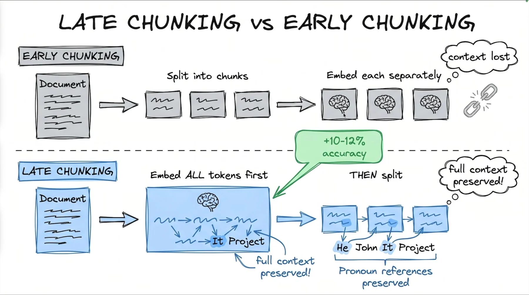
He / John / It / Project row under the split chunks is the payoff: coreference resolved before the split, so it survives it.Why it works is one sentence of transformer mechanics. When the model runs a forward pass over the whole document, attention lets every token see every other token. The token "He" in paragraph three is computed in the presence of "Steve Jobs" in paragraph one, so its vector already carries that association. Split those token vectors afterwards and each chunk's pooled vector inherits document-wide context that a standalone embedding of the same text could never have.
"each one of these chunks or vectors, because they're embeddings now, knows about the whole document." 06:33:38
Two terms this needs, because the course uses them without defining them. Token-level embeddings are the per-token vectors a transformer produces internally, before the model pools them into the single vector an embeddings API hands back. Pooling is that reduction: average (or otherwise combine) the token vectors falling inside a chunk's span into one chunk vector. In the script's ASCII diagram the late chunks are labelled Vector 1 (pooled), Vector 2 (pooled), Vector 3 (pooled) — the split produces embeddings, and each group of them is pooled down to one chunk vector, which is what lands in the database.
The claimed payoff: +10–12% accuracy on retrieval tasks. That figure appears on the slide's green callout, in the module docstring, in the comparison table and in takeaway #4. At 06:27:31 he says "10 to 20%" once — a verbal slip that conflicts with every written artefact, probably a merge with contextual retrieval's +15–20%. Use 10–12%.
3.2 The failure it fixes, made countable
The best asset in this chapter is a demo that proves the failure with a substring check and zero API calls. The test document is a Steve Jobs biography engineered so paragraph 1 names him and paragraphs 2–4 all open with "He".
# fcc-production-rag-part-6/03_late_chunking.py — demonstrate_early_chunking_problem()
# (the document literal keeps the source file's 4-space indentation — those spaces are
#  part of the text and they count toward chunk_size)
document = """
    Steve Jobs was born in San Francisco in 1955. He was adopted
    by Paul and Clara Jobs shortly after birth.

    He co-founded Apple Computer in 1976 with Steve Wozniak.
    The company started in his parents' garage. He served as CEO
    until 1985 when he was ousted from the company he created.

    He then founded NeXT Computer and acquired Pixar Animation Studios.
    These ventures would later prove instrumental in his return to Apple.

    He returned to Apple in 1997 and transformed it into one of the
    most valuable companies in the world. He introduced the iPod, iPhone,
    and iPad, revolutionizing multiple industries.
    """

# Simulate early chunking
splitter = RecursiveCharacterTextSplitter(
    chunk_size=200,
    chunk_overlap=0,  # No overlap to show the problem clearly
    separators=["\n\n", "\n", ". ", " "],
)

chunks = splitter.split_text(document)

for i, chunk in enumerate(chunks, 1):
    # Check if "Steve Jobs" appears in this chunk
    has_name = "Steve Jobs" in chunk
    pronoun_count = chunk.lower().count(" he ")

    print(f"\nChunk {i}:")
    print(f'  "{chunk.strip()[:80]}..."')
    print(
        f"  Contains 'Steve Jobs': {'Yes' if has_name else 'NO - Just pronouns!'}"
    )
    print(f"  Pronoun 'he' count: {pronoun_count}")
The run produces four chunks 06:30:34–06:31:35:
| Chunk | Opening text | Contains "Steve Jobs" | " he " count |
|---|---|---|---|
| 1 | "Steve Jobs was born in San Francisco in 1955…" | Yes | 1 |
| 2 | "He co-founded Apple Computer in 1976 with Steve Wozniak…" | NO – Just pronouns! | 3 |
| 3 | "He then founded NeXT Computer and acquired Pixar…" | NO | 0 |
| 4 | "He returned to Apple in 1997…" | NO | 1 |
Three of four chunks are unmatchable by name. The printed argument:
Chunks 2, 3, 4 only contain "he" - no "Steve Jobs"!

When embedding these chunks separately:
- Query: "What companies did Steve Jobs found?"
- Chunk 2 mentions "co-founded Apple" but says "He co-founded"
- Embedding of "He co-founded" won't match "Steve Jobs founded"

The pronoun "he" loses its referent when chunked separately.
The information is in the corpus and still not retrievable. That is the silent failure from invariant 4, in its purest form: nothing errors, nothing logs, the user just gets a worse answer. The generic version he narrates at 06:26:31 — spoken only, no artefact behind it — is a corporate announcement cut so that a chunk begins "He said it would take effect immediately" while the CEO who said it sits in the previous chunk. Same bug, and it is the shape most real corpora produce.
3.3 The two flows, side by side
visualize_chunking_approaches() prints the slide as a pair of ASCII flowcharts. Condensed here to one line per stage — the labels are verbatim from the script, the box art is not:
Original ASCII
EARLY CHUNKING (Traditional):
Full Document ─► [Split Text] ─► Chunk 1 | Chunk 2 | Chunk 3
                                    │        │        │
                                 [Embed]  [Embed]  [Embed]
                                    ▼        ▼        ▼
                                Vector 1 | Vector 2 | Vector 3

"Each chunk embedded INDEPENDENTLY - no cross-chunk context!"

LATE CHUNKING (Context-Preserving):
Full Document ─► [Embed FULL Document]
                      ▼
        Full Document Token Embeddings
        [tok1] [tok2] [tok3] ... [tok_n]
        "Each token has FULL document context via attention"
                      ▼
        [Split Embeddings by Position]
                      ▼
          Vector 1  |  Vector 2  |  Vector 3
          (pooled)     (pooled)     (pooled)

"Each chunk vector KNOWS about the whole document!"
"'He' in chunk 2 is embedded with knowledge that 'He' = 'Steve Jobs'"
"Each chunk as I say here is its own entity. It's embedded independently. So there's no cross-chunk context." 06:32:36
Isolation is the root cause and it is structural. No amount of better retrieval — no reranker, no query rewriting, no k=50 — fixes an embedding that was computed blind. That is invariant 1 again: quality is inherited forward and never recovered downstream.
The general law he draws from it, in two short quotes 06:27:31:
"everything is tied into context because large language models, they need context."
"doesn't matter how superior the model is, you will always end up with suboptimal results."
Model quality does not substitute for context quality. And the mental model to keep: "think of it as having the correct ideas, the full thoughts in each of the chunks."
3.4 The simulation, and what it does and does not prove
Here the course runs into a hard limitation and — to its credit — says so out loud. The OpenAI embeddings API does not expose token-level embeddings. You get one pooled vector per input string. True late chunking is therefore impossible with it. So the script fakes the effect by prepending a context string and re-embedding:
# fcc-production-rag-part-6/03_late_chunking.py — simulate_late_chunking()
embeddings = OpenAIEmbeddings(model="text-embedding-3-small")

chunk1 = "Steve Jobs was born in San Francisco in 1955. He was adopted by Paul and Clara Jobs shortly after birth."
chunk2 = "He co-founded Apple Computer in 1976 with Steve Wozniak. The company started in his parents' garage."

query = "What company did Steve Jobs found?"

# Early chunking: embed chunks separately
chunk2_embedding_early = embeddings.embed_query(chunk2)
query_embedding = embeddings.embed_query(query)
similarity_early = np.dot(chunk2_embedding_early, query_embedding)

# Late chunking simulation: embed chunk WITH context prepended
chunk2_with_context = (
    f"[Context: This is about Steve Jobs, founder of Apple] {chunk2}"
)
chunk2_embedding_late = embeddings.embed_query(chunk2_with_context)
similarity_late = np.dot(chunk2_embedding_late, query_embedding)

improvement = ((similarity_late - similarity_early) / similarity_early) * 100
print(f"\nImprovement: {improvement:.1f}%")

print("NOTE: This is a SIMULATION using context prepending.")
print("True late chunking uses token-level embeddings from")
print("models like Jina that support this natively.")
The result 06:34:39: 0.6857 → 0.6871, printed as Improvement: 0.2%.
"It has a small improvement. Nonetheless, it's still an improvement of 0.2%." 06:34:39
(The function also defines a document string and chunk1 and uses neither — they are scenery. Only chunk2 and query are ever embedded.)
His framing of what the win actually is, at 06:33:38: the query said "Steve Jobs", not "he" — and the retrieval still matched, because the chunk vector knows that "he" refers to Steve Jobs.
3.5 Actually implementing it
show_implementation_options() prints four options. Two of them have real problems in the current library versions and one of them is not late chunking at all — so read the code, then read the corrections.
Option 1 — Jina embeddings, native late chunking. As printed in the script:
# fcc-production-rag-part-6/03_late_chunking.py — OPTION 1, AS PRINTED (see warning below)
from langchain_community.embeddings import JinaEmbeddings

embeddings = JinaEmbeddings(
    model_name="jina-embeddings-v3",
    late_chunking=True  # Enable late chunking
)
Pros: native support, best quality. Cons: different model, may need an API key.
Also note the constraint the chapter never states:
Option 2 — contextual retrieval (§2 of this part), reprinted here as the model-agnostic alternative: context = generate_context(chunk, full_document), contextualized_chunk = f"{context} {chunk}", embed that. Pros: works with any embedding model. Cons: added LLM cost at indexing time.
Option 3 — Parent Document Retriever. The printed snippet has a stale import:
# fcc-production-rag-part-6/03_late_chunking.py — OPTION 3, AS PRINTED. Import is WRONG for LangChain 1.x
from langchain.retrievers import ParentDocumentRetriever
In LangChain 1.2.7 the langchain package exposes only agents, chat_models, embeddings, messages, rate_limiters, tools — there is no langchain.retrievers. The working import, and a working construction, come from the other repo:
# production-course-main-code/advanced_rag.py — the CORRECT import and a real working setup
from langchain_classic.retrievers import ParentDocumentRetriever
from langchain_classic.storage import InMemoryStore

parent_splitter = RecursiveCharacterTextSplitter(chunk_size=800, chunk_overlap=100)
child_splitter = RecursiveCharacterTextSplitter(chunk_size=200, chunk_overlap=20)

vectorstore = Chroma(
    collection_name="parent_child_demo",
    embedding_function=OpenAIEmbeddings(model="text-embedding-3-small"),
)
store = InMemoryStore()

retriever = ParentDocumentRetriever(
    vectorstore=vectorstore,
    docstore=store,
    child_splitter=child_splitter,
    parent_splitter=parent_splitter,
)

retriever.add_documents([long_doc])

# Search finds a SMALL child chunk...
child_docs = vectorstore.similarity_search(query, k=1)
# ...but the retriever returns the LARGE parent
parent_docs = retriever.invoke(query)
Small children give precise matching; the large parent gives the LLM room to reason. His description 06:37:42: the retriever walks the parent→child hierarchy and returns the parent, which carries the fuller context. (He calls it a "tree"; LangChain's implementation is really a docstore keyed by parent id, not a tree structure.)
Option 4 — overlap + summary headers. The poor man's version, and the one you should already be doing:
# fcc-production-rag-part-6/03_late_chunking.py — OPTION 4
splitter = RecursiveCharacterTextSplitter(
    chunk_size=500,
    chunk_overlap=100  # Overlap captures some context
)

# Add document summary to each chunk
for chunk in chunks:
    chunk.page_content = f"[From: {doc_title}] {chunk.page_content}"
Pros: simple, no extra cost. Cons: limited context preservation. Note that this is contextual retrieval with a template instead of an LLM — it gets you the document title into the vector for free, and nothing else. It is worth doing on day one of any project, because it costs a string format and buys the "which document?" half of the problem.
4. The scoreboard: five approaches, and the case for stacking them
4.1 The comparison table
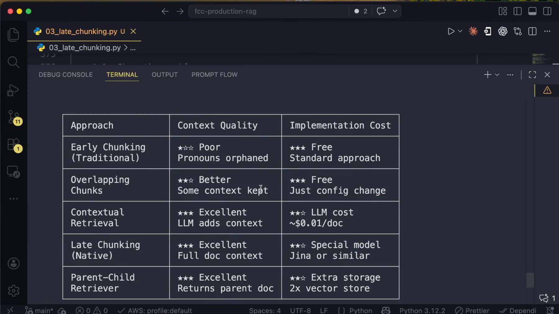
print_comparison(), not a slide — which is why you can reproduce it locally with uv run python 03_late_chunking.py. Read the two columns as quality vs what kind of cost: the last three rows all score three stars on quality, and they differ only in the currency they charge you — dollars per document, model lock-in, or storage.| Approach | Context quality | Implementation cost |
|---|---|---|
| Early chunking (traditional) | ★☆☆ Poor — pronouns orphaned | ★★★ Free — standard approach |
| Overlapping chunks | ★★☆ Better — some context kept | ★★★ Free — just config change |
| Contextual retrieval | ★★★ Excellent — LLM adds context | ★★☆ LLM cost ~$0.01/doc |
| Late chunking (native) | ★★★ Excellent — full doc context | ★★☆ Special model — Jina or similar |
| Parent-child retriever | ★★★ Excellent — returns parent doc | ★★☆ Extra storage — 2× vector store |
His gloss on orphaned 06:36:42: "they don't have attachment to a parent… they don't have any correlation pointing to the other piece of data that is contextually connected to it." On overlapping chunks: "It's better because we keep some context. Implementation cost is also free — you just need to configure a few things." On late chunking's cost column: the price is model lock-in, not dollars.
4.2 The accuracy scoreboard
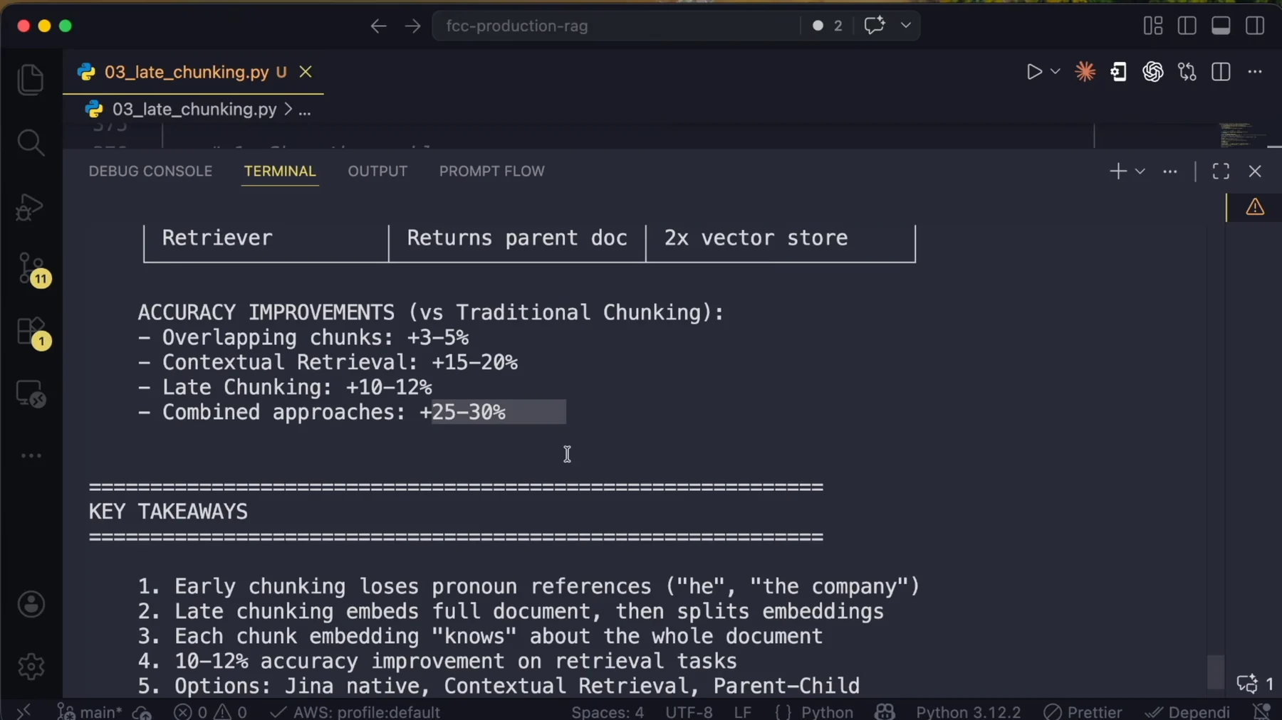
| Technique | Accuracy improvement vs traditional chunking |
|---|---|
| Overlapping chunks | +3–5% |
| Contextual retrieval | +15–20% |
| Late chunking | +10–12% |
| Combined approaches | +25–30% |
Note that the +15–20% here is higher than anything chapter 25 narrated about contextual retrieval — the two lessons quote different metrics (retrieval-failure reduction there, accuracy gain here) and never reconcile them. Two observations the course does not make explicitly, and both change what you should build:
4.3 Stack, don't choose
"It's not about just picking one strategy or approach and run with it." 06:38:42
06:38:42 His strategic point: at production level you want to pick all of these strategies so you end up with a hybrid system that uses all of them. The +25–30% row is the argument.
The code's own recommendation order — which is the single most actionable artefact in the chapter:
- Start with Contextual Retrieval (lesson 6.2) — works with any embedding model.
- If using Jina, enable native late chunking.
- Combine with Parent Document Retriever for best results.
- Always use meaningful chunk overlap (10–20%).
Read that as a build order, not a menu. Step 4 is free and you should already have it from Part 3. Step 1 is a change to your indexing job. Step 3 is a change to your retriever. Step 2 is a change to your embedding vendor — the most invasive change on the list, which is why it is conditional and second-to-last.
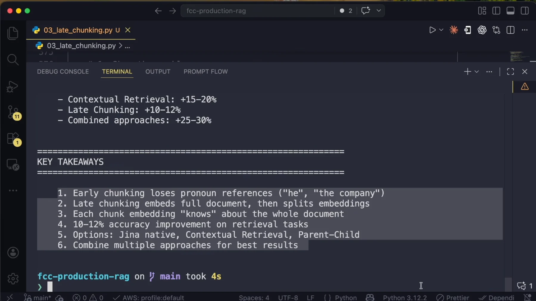
fcc-production-rag on main took 4s — this entire lesson runs in four seconds because only simulate_late_chunking() touches an API. The contextual-retrieval lesson before it took 19s, and that gap is the technique's cost profile in miniature.The six key takeaways, verbatim from the screen:
- Early chunking loses pronoun references ("he", "the company").
- Late chunking embeds full document, then splits embeddings.
- Each chunk embedding "knows" about the whole document.
- 10–12% accuracy improvement on retrieval tasks.
- Options: Jina native, Contextual Retrieval, Parent-Child.
- Combine multiple approaches for best results.
4.4 Where this hands off
The source chapter runs past its own subject: the last two and a half minutes of chapter 26 (06:39:44–06:42:04) are already the Agentic RAG concept slide, and it cuts off mid-sentence — "When the query comes in the…" — which the next chapter picks up. That material belongs to the agentic parts of this guide, not here, and the one-line preview is worth carrying forward:
"Currently production RAG isn't just a fixed pipeline that goes A, B, C… now at the center of everything you have an agent." 06:39:44
Everything in Part 14 is still a fixed pipeline: you decide at index time which technique to apply, and the query path executes the same steps every time. The next frontier is a retrieval loop that evaluates its own results and re-queries when they are bad — which is where this guide goes next.
5. Diagnostics you can run this week
Two procedures, both cheap, both giving you evidence instead of vibes.
5.1 Count the orphans in your own corpus
Generalised from the Steve Jobs demo. Costs nothing — no API calls.
- Split a representative document with your production splitter settings (not the
demo's chunk_overlap=0).
- For each chunk, test whether the canonical entity name appears in it.
- Count pronouns and definite references as separate columns:
he,him,his,she,
her, they, them, it, the company, the report. Use word-boundary regex, not count(" he ") — see the bug in §3.2.
- Any chunk with pronouns but no name is a chunk your embeddings cannot match by name.
In the demo that is 3 of 4. If it is a meaningful fraction of your corpus, contextual retrieval will pay for itself.
5.2 Simulate the benefit before buying a new embedding model
- Pick a chunk that begins with a pronoun, and a query that names the entity.
- Embed the query and the standalone chunk; take the dot product → baseline.
- Prepend a one-line context string, re-embed, dot product again.
improvement = ((late - early) / early) * 100.- Expect a small number (0.2% in the course's run). This proves direction only. If you
want magnitude, run a real retrieval eval over a labelled query/passage set — the measurement discipline from Part 7 — not a single-pair dot product.
5.3 Reproduce the three lessons
cd fcc-production-rag-part-6           # requires OPENAI_API_KEY in .env
uv run python 01_long_context_vs_rag.py   # cost math, latency, framework, hybrid demo
uv run python 02_contextual_retrieval.py  # ~19s, real LLM + embedding calls
uv run python 03_late_chunking.py         # ~4s, three embed_query calls in the simulation
Environment, from the repo metadata rather than the README (which claims Python 3.10+ and is wrong): .python-version = 3.13 and pyproject.toml requires-python >= 3.13, pinning langchain>=1.2.0,<2.0.0, langchain-openai>=1.1.0, langchain-chroma>=1.1.0, langchain-text-splitters>=1.1.2, openai>=2.32.0, tiktoken>=0.12.0, networkx, python-dotenv. requirements.txt adds what pyproject.toml omits — chromadb>=1.5.0, langchain-classic>=1.0.0, langgraph>=1.1.0 — and carries the header rule "use langchain-chroma, NOT langchain-community" for the vector store. The screen recording shows Python 3.12.2 in VS Code, so README, pyproject.toml and the recorded environment all disagree. Trust pyproject.toml.
6. Decisions to make
Work down this list in order. Each row is a decision with a default, not a suggestion.
| # | Decision | Default / trigger |
|---|---|---|
| 1 | RAG or long context for this corpus? | Corpus <50K tokens and <100 queries/day and whole-document questions → long context. Otherwise RAG. Anything ambiguous → RAG, because it degrades gracefully as the corpus grows. |
| 2 | Do the scale arithmetic before committing. | Compute cost/query, then ×volume×30. If the monthly delta is smaller than an engineer-hour, either design is fine; once it is not, the architecture is a financial decision, not a taste one. |
| 3 | Budget against the *effective* context limit. | 60–70% of the advertised window. On a 1M model, plan for 600–700K. |
| 4 | Add the hybrid selector pattern. | If users ask whole-document questions about one of many documents: k=1 retrieval → load full document → answer. Cheapest big win in this part. |
| 5 | Run the orphan count (§5.1). | If a large minority of chunks carry pronouns without their referent, turn on contextual retrieval. Measure the fraction; do not guess it. |
| 6 | Turn on contextual retrieval if any trigger fires. | Context in headers/titles · pronoun-referenced entities · multi-source corpora. |
| 7 | Budget contextualization honestly. | $0.01–$0.05/doc is a floor. Real cost ≈ chunks × document length in input tokens. Add prompt caching and batch APIs before running it over a large corpus — the course covers neither. |
| 8 | Make contextualization asynchronous. | 1–2 s/chunk. Queue it. Never inline it in an upload request. |
| 9 | Persist original_chunk and context_prefix in metadata. | Embed the contextualized text, cite the original, audit the prefix. Non-negotiable. |
| 10 | Set title or source on every loaded document. | create_contextual_chunks() falls back to the literal string "Unknown Document" and generates every prefix against it. Silent, and it poisons the whole index. |
| 11 | Index the contextualized text into BM25 too. | Takeaway #6. Anthropic's 49% figure is embeddings + contextual BM25, not embeddings alone. |
| 12 | Plan for 20–30% chunk growth. | Storage impact is minimal; prompt impact is not. A top-5 retrieval now stuffs ~25% more text into every answer prompt. Re-check the token budget from Part 9. |
| 13 | Late chunking: only with a model that truly supports it. | Verify the request body actually carries late_chunking. The LangChain community wrapper silently drops it. |
| 14 | Check your documents fit the embedder's window. | Late chunking needs the whole document in one forward pass. Read the model card for the real limit; past it you are segmenting, and choosing segment boundaries, again. |
| 15 | Layer Parent-Child on top of whichever you chose. | It fixes a different axis (what is returned) and costs 2× vector storage. Use langchain_classic.retrievers, not langchain.retrievers. |
| 16 | Always keep 10–20% chunk overlap. | +3–5% for a config change. There is no argument against it. |
| 17 | Measure your own numbers. | Every figure in this part — 1,200×, 25×, 49%, 67%, +10–12%, +15–20%, +25–30% — is directional. "These are just benchmarks. So you have to test on your own." 06:24:26 |
The three techniques in this part all buy the same thing: a chunk that can be found by a question phrased the way a human would phrase it. Long context buys it by never splitting. Contextual retrieval buys it by writing the missing words in. Late chunking buys it by embedding before splitting. Pick by cost and constraint, not by novelty — and remember that the boring free one, 10–20% overlap, is already on the scoreboard.