
Scaling: Index Tuning, HNSW and When to Shard
HNSW's M and ef, recall vs latency presets, vertical scaling first and when to shard.
Everything up to here made your system good. This part makes it survive growth — and it starts with the observation that growth breaks RAG in a way you will not see in your test suite.
The failure arc is always the same 03:12:59. You develop against a few thousand documents. Queries come back instantly. You ship. Production has a hundred thousand documents, or a million, or ten million — the instructor's own answer to "how many?" is "who knows?" — and two things go wrong at once:
- Queries get slow. Milliseconds become seconds.
- Queries get wrong — the instructor's own "or worse" — because the index was never
configured for this scale.
The second is the one that will cost you a quarter. An approximate index that is under-tuned does not raise an exception, does not log a warning, and does not return fewer results. It returns k documents that look exactly like the right answer's shape and are simply not the true nearest neighbours. This is invariant 4 of the mental model — failures are silent — showing up at the infrastructure layer, and it is why this part comes after observability (Part 7) rather than before: every trigger in this part is a number you must already be measuring.
In the two-phase picture, this part modifies exactly two boxes: Store + Index in Phase A and Retrieve in Phase B. It changes no chunking, no embeddings, no prompts. That is precisely what makes it dangerous — you can degrade retrieval quality without touching a single line of application code.
Tuning the index is the only optimisation in this guide that can make your answers worse while every dashboard stays green.
Embedding is not indexing
The seed planted back in Part 1 has to be dug up now, because the rest of this part is unintelligible without it. A vector store does two independent things, and people routinely confuse them:
- Embedding decides where a vector lands in space. It is a property of the model.
- Indexing decides how you find the neighbours of a point once they are all in that
space. It is a property of the data structure built on top of the vectors.
They are orthogonal. You can have perfect embeddings and a badly tuned index (correct geometry, wrong neighbours returned) or garbage embeddings and a perfect index (you retrieve the true nearest neighbours of a meaningless point, flawlessly). The two failure modes look identical from the outside — "the right chunk wasn't retrieved" — and have completely different fixes.
| Property | Decides | Set at | Cost to change | Failure signature |
|---|---|---|---|---|
| Embedding model | where each vector is | index time, then frozen forever | re-embed the entire corpus: full API bill + full rebuild | silent incomparability (invariant 2); mismatched dims fail loudly, same-dims-different-model fails silently |
| Index type + M | the graph you search through | index build time | rebuild the graph over the existing vectors — no re-embedding, no API cost | recall quietly below 100%; results plausible but not optimal |
| Search effort (ef) | how hard you look on this query | query time on pgvector, collection level on Chroma | free-to-cheap — change a setting, no rebuild | recall drops as the corpus grows, with zero code change |
That third row is the whole reason this part is worth reading. There is one knob in your entire retrieval stack that costs nothing to change, requires no rebuild, and moves accuracy several points. Most teams never touch it because they don't know it exists.
HNSW, in the amount of detail you actually need
Most vector databases index with HNSW — Hierarchical Navigable Small World graphs — or something closely related. The instructor names four: Pinecone, pgvector, Chroma and Qdrant 03:12:59. (Qdrant is named exactly once in the seven and a half hours of the course and never returned to.)
The essential idea: instead of comparing your query against every stored vector — exact but O(n), unusable at a million vectors — HNSW builds a graph where each vector is a node connected to a handful of its neighbours, arranged in layers. A search enters at the sparse top layer, greedily walks toward the query, drops a layer, walks again, and finishes with a fine-grained walk at the bottom. You visit a few hundred nodes instead of a million.
The price is in the name of the family: ANN — approximate nearest neighbour. The graph walk can get stuck in a local neighbourhood and miss a genuinely closer vector that lives one unexplored edge away. The approximation is not a bug you can eliminate; it is the trade you make in exchange for sub-linear search. What the two parameters do is buy back accuracy — one with memory, one with time.
The course is explicit and, I think, correct about scope:
"You don't need to understand the algorithm deeply … But you do need to understand the two parameters that control everything." 03:12:59
Take that at face value with one caveat: the two-knob abstraction is sufficient for operating an index. It is not sufficient for debugging pathological recall, where things like the distance metric, vector normalisation and the layer-assignment probability start to matter. Ninety-plus percent of production tuning is M and ef.
Parameter 1 — M, the number of friends each vector has
M is the maximum number of connections (edges) per node in the graph. Picture the vector space as a graph of nodes with edges between them; M is how many edges each node gets.
The analogy the course uses is the one worth memorising:
"think of it like social network. Low m … means everyone knows eight people. High m means everyone knows 64 people." 03:15:03
More friends means any target can be reached in fewer hops, so the greedy walk finds the true neighbourhood more reliably. It also means you store all those edges — in RAM, forever, for every vector in your corpus. And building the graph is slower, because each insertion has to choose and maintain more connections.
| M band | Values | Index size | Build speed | Accuracy |
|---|---|---|---|---|
| Low | 8–16 | smaller | faster builds | lower |
| Default | 16 | balanced | balanced | balanced |
| High | 32–64 | larger | slower builds | higher |
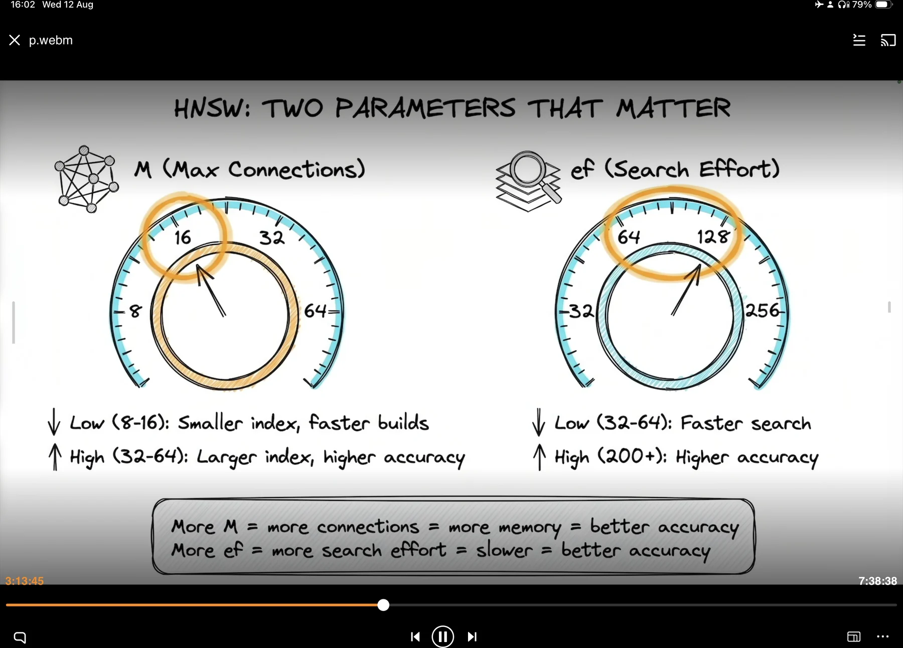
Slide 11 draws M as a dial with ticks at 8 / 16 / 32 / 64 and circles 16 as the default, under the one-line law:
"More M = more connections = more memory = better accuracy." — slide, 3:13:45
Note that raising M costs you twice: a bigger resident index and a slower build or re-index 03:14:01. That double cost is the reason the tuning advice further down moves ef first and M last.
Parameter 2 — ef, how hard the search tries
ef is the size of the dynamic candidate list maintained during a search 03:15:03. When the traversal walks the graph, it keeps a working set of the best candidates found so far and keeps expanding from them; ef is how large that working set is allowed to get before the search settles. A bigger list means more of the graph gets explored, more chances to escape a local optimum, better recall — and more distance computations per query.
| ef band | Values | Search speed | Accuracy |
|---|---|---|---|
| Low | 32–64 | faster | lower |
| Default | 64–128 | balanced ("that nice balanced effect") | balanced |
| High | 200+ | slower | higher |
Slide 11's dial for ef runs 32 / 64 / 128 / 256 with the 64–128 zone circled, and states the top band as "High (200+): Higher accuracy". The narration says "between 200 and 500" 03:15:03. Those do not actually contradict each other — the slide's band is open-ended and its dial simply stops drawing at 256. The number that matters is 200, because that is what the high-accuracy preset uses; treat anything past 256 as off-dial territory you only enter holding a recall measurement.
"More ef = more search effort = slower = better accuracy." — slide, 3:13:45
The asymmetry that governs everything
The slide draws M and ef as two identical dials. They are not identical, and the difference is the most actionable thing in this chapter:
- M is baked in at build time. Changing it means rebuilding the index.
- ef is not. It is set after the graph exists and can be raised without re-embedding
anything.
How cheap "not baked in" is depends on your store, and it is worth knowing before you plan around it:
- pgvector: truly per-request.
SET hnsw.ef_searchis a session setting, so different
queries on different connections can use different values.
- Chroma: a collection-level setting. You choose it at collection creation, and on
current versions you can change it afterwards with collection.modify(...). What you cannot do is vary it per query.
- Pinecone: not exposed at all.
So: when accuracy is short, raise ef first. It is reversible, cheap to try, and needs no re-embedding. Only raise M — and pay for a rebuild plus permanent RAM — when ef alone can't get you there.
Three parameters wearing two names
The single nastiest naming trap in this material. "ef" on the slide means search effort, but the pgvector example below sets ef_construction, and the preset table's "ef" is a search value. Three distinct things:
| Parameter | When it applies | Effect | Reversible? |
|---|---|---|---|
m | build | edges per node; graph density | rebuild required |
ef_construction | build | how hard the builder searches while inserting each vector — graph quality, permanently | rebuild required |
ef_search | search | how hard the traversal looks | yes, without a rebuild |
ef_construction is not a performance knob for your users; it is a quality knob for the graph itself. Set it too low and you produce a permanently mediocre graph that no amount of search-time ef can fully rescue. Set it high and you pay once, at build time, in wall-clock.
The production trade-off: pick two
"unfortunately you can't have all three working together" 03:16:04
Three corners — Accuracy, Speed, Memory — and the words in the middle of the slide are PICK 2. This is invariant 5 of the mental model instantiated at the index layer, and the three corners map one-to-one onto the guide's three budgets: accuracy is the quality budget, speed is the latency budget, and memory is the money budget (RAM is the line item you rent by the month). Every index decision in this part is a transfer between those three accounts.
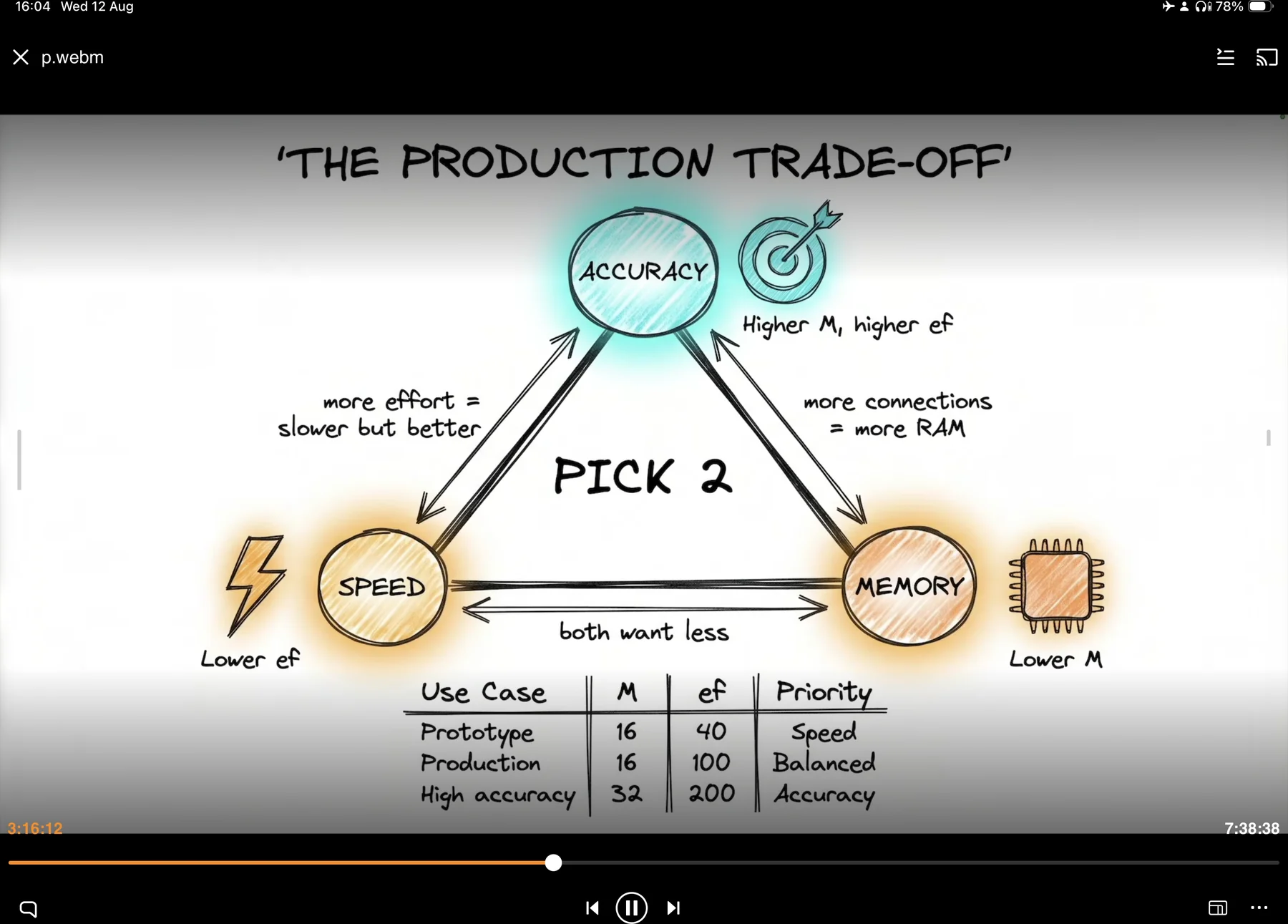
The three levers, stated as if-then-pay 03:16:04:
| Your goal | Action | The price you pay |
|---|---|---|
| High accuracy | increase both M and ef | memory and speed |
| Faster queries | decrease ef | accuracy |
| Smaller index | decrease M | accuracy |
The slide's edge and corner labels encode the geometry, and are worth reading carefully:
- Speed ↔ Accuracy: "more effort = slower but better" (that edge is ef; the SPEED corner is
annotated "Lower ef")
- Memory ↔ Accuracy: "more connections = more RAM" (that edge is M; the MEMORY corner is
annotated "Lower M")
- Speed ↔ Memory: "both want less"
- And beside ACCURACY: "Higher M, higher ef" — the only corner that costs you both
That third edge is the insight. Speed and memory-frugality are not in tension with each other — they both want smaller, cheaper settings. The genuine tension is one-against-two: accuracy versus the pair. Which reframes the whole exercise: you are not balancing three things, you are deciding how much speed and RAM you are willing to spend to buy recall.
"usually pick two, you can't pick three." 03:16:04
The three presets
This is the practical output of the chapter — the table at the bottom of slide 12, also read aloud 03:16:04–03:17:04:
| Use case | M | ef | Priority |
|---|---|---|---|
| Prototype | 16 | 40 | Speed |
| Production | 16 | 100 | Balanced |
| High accuracy | 32 | 200 | Accuracy |
Look at the shape of that advice rather than the numbers. M moves 16 → 16 → 32. ef moves 40 → 100 → 200. Across the entire range from throwaway prototype to accuracy-critical system, M changes exactly once and ef changes by 5×. The presets are themselves an argument for "tune ef, leave M alone" — which is exactly what the build-time/search-time asymmetry predicts.
Two footnotes on the numbers:
- Prototype ef = 40 sits inside the stated low band (32–64) but is not one of the dial's
ticks. Read it as "deliberately cheap", not as a magic constant.
- The instructor hedges explicitly — they are "really good starting points" 03:17:04 to be
checked against your own use case, not answers. Values to measure from.
Setting the parameters, per database
Three vendors, three genuinely different surfaces — and one of them has no surface at all.
pgvector — SQL, twice
You write it once at build time in DDL, and once at query time:
-- build time: M and ef_construction are baked into the index
CREATE INDEX ON documents
  USING hnsw (embedding vector_cosine_ops)
  WITH (m = 16, ef_construction = 64);

-- query time: raise search effort for higher accuracy (slower)
SET hnsw.ef_search = 100;
vector_cosine_ops is the cosine-distance operator class — the operator class has to match the distance operator you actually search with (<=> for cosine), or the planner will ignore the index and sequential-scan the table. Note also that the DDL's m = 16, ef_construction = 64 are pgvector's own defaults, so that statement is really documenting an intention rather than changing behaviour; the line that changes behaviour is the second one.
The second statement is a session GUC: it applies to subsequent queries on that connection. In a pooled application that is a trap — set it once at startup and it will silently apply to whichever connection happened to be checked out at the time and no others. Set it on every checkout, or scope it to the transaction with SET LOCAL hnsw.ef_search = 100 inside the transaction that runs the search. (The pooling point and the operator-class point are mine, not the course's; the pooling one is the most common way this setting fails to apply in production.)
Chroma — a metadata dictionary at collection creation
Chroma exposes HNSW settings as hnsw:-prefixed entries in the collection's metadata dict, set when the collection is created:
# Chroma native client — HNSW settings live in collection metadata
collection = client.create_collection(
    name="my_collection",
    metadata={
        "hnsw:space": "cosine",
        "hnsw:M": 16,
        "hnsw:construction_ef": 100,
        "hnsw:search_ef": 100,
    },
)
And through the LangChain wrapper the whole course actually uses:
from langchain_chroma import Chroma

vectorstore = Chroma.from_documents(
    documents=docs,
    embedding=embeddings_model,
    persist_directory="./chroma_db/",
    collection_metadata={
        "hnsw:space": "cosine",
        "hnsw:M": 16,
        "hnsw:construction_ef": 100,
        "hnsw:search_ef": 100,
    },
)
Three things about this that the source does not tell you and that are worth more than the snippet itself. All three were checked against the versions this guide's repo pins, chromadb 1.4.1 / langchain-chroma 1.1.0:
1. Chroma's untouched defaults are already the production preset — except the metric. A collection created with no HNSW metadata at all comes out as {space: "l2", ef_construction: 100, ef_search: 100, max_neighbors: 16, …}. max_neighbors is M. So the course's production row (M = 16, ef = 100) is not a change to Chroma, it is a restatement of what Chroma already does. The one thing worth setting explicitly is hnsw:space, which defaults to L2, not cosine. With OpenAI's unit-normalised embeddings L2 and cosine rank identically, so this does not break ranking — but it does change the score scale, which is exactly why Part 4 insists a distance threshold is never portable between stores.
2. You can read back what Chroma actually built. Do not trust that your settings landed — verify:
# Verified on chromadb 1.4.1: legacy hnsw:* keys are translated into the modern config
print(vectorstore._collection.configuration_json["hnsw"])
# {'space': 'cosine', 'ef_construction': 100, 'ef_search': 100, 'max_neighbors': 16, ...}
3. A mistyped key fails in two completely different ways. A key inside the hnsw: namespace that Chroma does not recognise — hnsw:m in lower case, or hnsw:ef_search when the legacy name is hnsw:search_ef — makes create_collection raise InvalidArgumentError: Failed to parse hnsw parameters from segment metadata. A key that misses the prefix entirely — "M": 16 — is accepted, stored as ordinary collection metadata, and does absolutely nothing. The loud failure is the lucky one.
Newer Chroma also accepts a structured configuration instead of the legacy metadata keys, which langchain_chroma surfaces as collection_configuration=. It is the same three numbers under better names, and unlike the metadata dict it can be updated on an existing collection:
# modern equivalent; max_neighbors is M, and modify() works after creation
collection = client.create_collection(
    name="my_collection",
    configuration={"hnsw": {"space": "cosine", "ef_construction": 100,
                            "max_neighbors": 16, "ef_search": 100}},
)
collection.modify(configuration={"hnsw": {"ef_search": 300}})  # no rebuild
That modify call is the closest Chroma gets to pgvector's per-request SET: it changes the search effort of an existing collection without re-embedding anything. It is also the only sanctioned way to change ef after the fact — reopening a collection with different metadata does not work, which is the next callout.
Pinecone — no knobs
"you don't have to worry about this, but you can control the number of results. In this case, top K." 03:18:05
Pinecone auto-tunes HNSW against your pod type. You pick the pod; Pinecone picks M and ef. The entire tuning surface of this part is replaced by two decisions: which pod and what top_k.
That is sold as convenience, and mostly it is. But notice what it costs: it is the control column of the managed/self-hosted trade being spent. If you need deterministic, reproducible index behaviour — for example a recall benchmark in an eval suite that must not move underneath you between runs — autotuning is a limitation, not only a feature. And note that the pod framing describes Pinecone's pod-based tier; the serverless tier that Part 9's own recommendation ladder picks for 100 K–1 M vectors has no pod to size, which collapses the surface further, to top_k alone.
| Vendor | Build-time surface | Search-effort surface | Who chooses |
|---|---|---|---|
| pgvector | WITH (m=…, ef_construction=…) in DDL | SET hnsw.ef_search = …, per session or per transaction | you, fully |
| Chroma | collection_metadata={"hnsw:M": …, "hnsw:construction_ef": …} at creation | hnsw:search_ef at creation, or modify(configuration=…) later — never per query | you, at creation |
| Pinecone | none — pod type | none — only top_k | Pinecone |
| Qdrant | HNSW config (named once in the source, never expanded) | — | you |
The code the course never wrote
A blunt fact worth stating plainly: neither course repo contains a single HNSW setting. Searching both production-course-main-code/ and fcc-production-rag-part-6/ for hnsw, ef_search, ef_construction, collection_metadata and create index returns nothing. This chapter is 100% slides — no editor is opened, nothing is executed.
So here is the file it should have edited. Every Chroma construction in the repo runs on stock defaults:
# production-course-main-code/vector_stores.py:50-58, as shipped
def chroma_basics():
    with tempfile.TemporaryDirectory() as tmpdir:
        # create vector store from documents
        vectorstore = Chroma.from_documents(
            documents=SAMPLE_DOCS, embedding=embeddings_model, persist_directory=tmpdir
        )
        print(
            f"Vector store created {vectorstore._collection.count()} documents and persisted."
        )
No collection_metadata — so every store in chroma_basics(), similarity_search_with_scores(), metadata_filtering(), as_retriever(), persist_chroma() and the exercise at the bottom of the file is built at M = 16, ef_construction = 100, ef_search = 100, L2. At eight sample documents that is entirely correct behaviour: the graph is far smaller than the candidate list, so every search is effectively exhaustive and recall is 1.0 by construction. It is also why you will never observe an index-tuning problem in this repo, which is precisely the "dev is a lie" trap the chapter opens with.
The tuned version of the same function — the one-line delta:
# vector_stores.py, tuned: the production preset stated explicitly at collection creation
def chroma_basics_tuned():
    with tempfile.TemporaryDirectory() as tmpdir:
        vectorstore = Chroma.from_documents(
            documents=SAMPLE_DOCS,
            embedding=embeddings_model,
            persist_directory=tmpdir,
            collection_metadata={          # <-- the whole of Part 8, in one kwarg
                "hnsw:space": "cosine",
                "hnsw:M": 16,
                "hnsw:construction_ef": 100,
                "hnsw:search_ef": 100,
            },
        )
        cfg = vectorstore._collection.configuration_json["hnsw"]
        print(f"{vectorstore._collection.count()} docs indexed with {cfg}")
k is not ef — and ef must be ≥ k
Not stated in the source, and it bites people. The retriever's k and the index's ef are different numbers at different layers:
# vector_stores.py:129-131 — k is an application-layer setting
retriever = vectorstore.as_retriever(
    search_type="similarity", search_kwargs={"k": 3}
)
k is how many documents you want back. ef is how many candidates the graph walk is allowed to consider on the way to finding them. The candidate list has to be at least as large as the result set, so ef_search ≥ k always, and ef_search meaningfully larger than k is where the accuracy actually comes from. If you use the MMR retriever in the same file, note that fetch_k raises the real result-set demand:
# vector_stores.py:141-144 — MMR fetches 5, returns 3 diverse
mmr_retriever = vectorstore.as_retriever(
    search_type="mmr",
    search_kwargs={"k": 3, "fetch_k": 5},  # fetch 5 docs and return 3 diverse
)
With fetch_k=5 the index must produce five candidates, so ef_search=40 gives you a comfort margin of 8× and ef_search=100 gives you 20×. Where this goes wrong is at the other end: a reranking pipeline (Part 6) that retrieves k=100 to rerank down to 5 is asking the index for 100 results with a candidate list of 100 — a ratio of 1.0, which is the worst possible recall configuration. If you rerank, raise ef.
Measure it yourself — a recall harness that needs no API key
The chapter asserts that ef buys accuracy and never shows it. This does, offline, in about thirty seconds. DeterministicFakeEmbedding stands in for a real embedding model so the index is the only variable, and a brute-force cosine scan over the same vectors supplies the ground truth the ANN result is scored against.
# Original: an offline recall harness. Needs chromadb + langchain-chroma + numpy.
import tempfile

import numpy as np
from langchain_chroma import Chroma
from langchain_core.embeddings import DeterministicFakeEmbedding

PRESETS = {
    "prototype":     {"hnsw:space": "cosine", "hnsw:M": 16, "hnsw:construction_ef": 100, "hnsw:search_ef": 40},
    "production":    {"hnsw:space": "cosine", "hnsw:M": 16, "hnsw:construction_ef": 100, "hnsw:search_ef": 100},
    "high_accuracy": {"hnsw:space": "cosine", "hnsw:M": 32, "hnsw:construction_ef": 200, "hnsw:search_ef": 200},
}


def effective_hnsw_config(vectorstore: Chroma) -> dict:
    """Read back what Chroma built, not what you asked for."""
    return vectorstore._collection.configuration_json["hnsw"]


def recall_at_k(vectorstore, embeddings, texts, queries, k=5) -> float:
    matrix = np.array(embeddings.embed_documents(texts))
    matrix /= np.linalg.norm(matrix, axis=1, keepdims=True)
    hits = 0
    for query in queries:
        qv = np.array(embeddings.embed_query(query))
        qv /= np.linalg.norm(qv)
        exact = {texts[i] for i in np.argsort(-(matrix @ qv))[:k]}  # brute force = ground truth
        approx = {d.page_content for d in vectorstore.similarity_search(query, k=k)}
        hits += len(exact & approx)
    return hits / (k * len(queries))


embeddings = DeterministicFakeEmbedding(size=1536)
texts = [f"document number {i}" for i in range(2000)]
queries = texts[::200]

for name, preset in PRESETS.items():
    with tempfile.TemporaryDirectory() as tmpdir:
        store = Chroma.from_texts(
            texts=texts, embedding=embeddings,
            persist_directory=tmpdir, collection_metadata=preset,
        )
        cfg = effective_hnsw_config(store)
        print(
            f"{name:14s} M={cfg['max_neighbors']:3d} ef_search={cfg['ef_search']:4d} "
            f"recall@5={recall_at_k(store, embeddings, texts, queries):.2f}"
        )
Typical output on 2 000 vectors (chromadb 1.4.1; the exact figures move a point or two between runs):
prototype      M= 16 ef_search=  40 recall@5=0.90
production     M= 16 ef_search= 100 recall@5=0.97
high_accuracy  M= 32 ef_search= 200 recall@5=1.00
Three things to take from it. First, the presets are real: the ordering is exactly what the slide claims. Second — and this is the point of the whole part — all three runs returned five documents and raised nothing. The prototype preset lost one true neighbour in ten and told you nothing about it. Third, note how noisy 10 queries × k = 5 is: fifty judgements is not enough to distinguish a two-point recall change, which is your first lesson about golden-set size. Random Gaussian vectors in 1536 dimensions are also a deliberately hard case for ANN, so read these numbers as a lower bound, not as a forecast for your corpus.
When to scale: four symptoms, four diagnoses
Before you buy anything, name the symptom. The course's table 03:18:05–03:19:07:
| Symptom | Likely cause | Solution |
|---|---|---|
| Queries take ≥ 100 ms | index is too large for memory | add more RAM, or shard |
| Insert latency spiking | write bottleneck | scale writes separately |
| Out-of-memory errors | index doesn't fit what you're doing | bigger instance, or shard |
| Accuracy dropping | ef_search too low for the new scale | increase ef, or shard |
Three observations the table doesn't make for you.
The 100 ms threshold is a vector-search threshold, not an end-to-end one. Your users' p95 is dominated by generation, which is measured in seconds. A 100 ms retrieval step is therefore not a latency emergency for the user — it is a diagnostic that your index has stopped fitting comfortably in RAM. Treat it as a memory alarm wearing a latency costume.
Row 4 is the important one and it is easy to miss. An ef_search that was correct at 100 K vectors is not correct at 10 M vectors. A fixed candidate list explores a shrinking fraction of a growing graph, so recall silently decays as the corpus grows. Nothing in your code changed. Nothing errors. Your answers just get slightly worse every week.
Growth degrades retrieval quality by itself. Re-tune ef when the corpus grows; yesterday's configuration is not evidence about today's.
Row 2 is the only fix that isn't about RAM. "Scale writes separately" points at read/write separation — a dedicated write path, replicas for reads, batched inserts — and the source names it and never expands it. No replica topology, no queue design, no batching guidance is given anywhere in the chapter. Treat it as a pointer, not a design. Its one practical implication you can act on today: measure insert latency on its own series, because a write bottleneck is invisible in a query-latency dashboard.
You cannot act on any of this without instrumentation
Every row above is a measurement. This is why Part 7 comes before Part 8 in this guide even though the course orders them the other way: the triggers are useless if you can't see them. The repo's metric collector is the right shape and the wrong scope —
# production-course-main-code/monitoring.py:95-105 — the summary the repo produces
    def get_summary(self) -> dict:
        avg_latency = (
            self.metrics["latency_sum"] / self.metrics["latency_count"]
            if self.metrics["latency_count"] > 0
            else 0
        )
        error_rate = (
            self.metrics["errors_total"] / self.metrics["requests_total"]
            if self.metrics["requests_total"] > 0
            else 0
        )
Two gaps for our purposes. First, InstrumentedLLM times the LLM call, not the retrieval call — the 100 ms signal you need is invisible to it. Second, it reports avg_latency_ms, and an average hides exactly the tail you are hunting: an index that has half-spilled out of RAM shows a fine mean and a catastrophic p95.
Instrument the retriever itself, and keep percentiles:
# Original: retrieval-only timing, built on the repo's MetricsCollector shape.
# Wrap the retriever, not the chain — the index signal lives here.
import time
from collections import deque
from statistics import quantiles


class TimedRetriever:
    def __init__(self, retriever, window: int = 2000):
        self.retriever = retriever
        self.samples_ms: deque[float] = deque(maxlen=window)

    def invoke(self, query: str):
        start = time.perf_counter()
        docs = self.retriever.invoke(query)          # never swallow: no try/except here
        self.samples_ms.append((time.perf_counter() - start) * 1000)
        return docs

    def p95_ms(self) -> float:
        if len(self.samples_ms) < 20:
            return 0.0                                # too few samples to have a tail
        return quantiles(self.samples_ms, n=20)[-1]   # 19th cut point = 95th percentile
Alert on p95_ms() >= 100. That is the course's scale trigger, made measurable. The bounded deque matters more than it looks: an unbounded sample list in a long-running API process is a slow memory leak inside your memory-pressure detector.
And for row 4 — accuracy decay — there is no timing signal at all. You need the golden set from Part 7 (question → expected chunk) replayed on a schedule with recall@k tracked as a time series, wired into the CI regression gate of Part 13. Without it, row 4 is undetectable by construction; the harness in the toggle above is the smallest version of it that runs.
Vertical before horizontal
Vertical scaling — buy RAM, change nothing
Definition: "just get bigger machine, more RAM, more CPU" 03:20:08. The worked example:
| RAM | Vectors | Query latency | |
|---|---|---|---|
| Before | 8 GB | 100 K | ~50 ms |
| After | 32 GB | 100 K | ~10 ms |
Same data. Same index. Same code. 5× faster. The mechanism is stated in four words:
"That means index fits in memory." 03:20:08
That sentence is the physics of this entire part. Vector search performance is, first and before anything else, a question of whether the index fits in RAM. Everything else — M, ef, sharding, vendor choice — is downstream of that one binary condition. When the index spills, your graph walk starts touching disk on random access patterns, which is the worst thing you can do to a storage device.
The three conditions the instructor attaches to vertical scaling 03:20:08: you are under 5–10 M vectors, your budget stretches to a bigger instance, and — the one people skip — simplicity matters to you more than cost. That third condition is a real decision, not filler: a bigger box is often the expensive answer and still the right one, because the cheaper answers all cost engineering time.
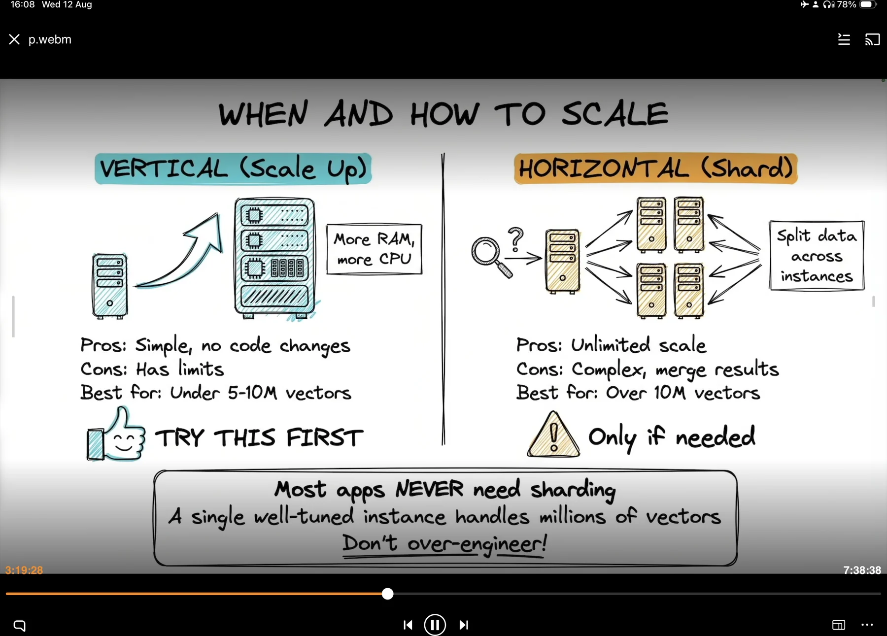
Slide 13's card for vertical: Pros "Simple, no code changes" · Cons "Has limits" · Best for "Under 5-10M vectors" · badge "TRY THIS FIRST".
"vertical scaling is the easiest, the quickest one. So you would always try this first." 03:20:08
Horizontal scaling — split the data, inherit a merge problem
Definition: splitting your data across multiple instances, each holding a slice 03:20:08–03:21:10. Pros: unlimited scale. Cons: complexity — "because you're merging results and all of that" 03:21:10. Best for: over 10 million vectors. Badge: "Only if needed".
The cost of sharding is not the servers. It is correctness. Every query now fans out to N shards and something has to merge N result sets into one ranking, which introduces failure modes that simply do not exist on a single instance:
- Each shard must return more than your final
k(typicallykper shard, then merge and
truncate) or you lose true top-k documents that happened to cluster in one shard.
- Scores must be comparable across shards. With cosine distance they usually are; with any
score normalisation, hybrid fusion (Part 6's RRF) or per-shard reranking, they frequently are not.
- Recall becomes non-uniform: a shard whose slice happens to be denser has a harder search
problem at the same ef.
- One slow or restarting shard degrades every query, not one in N.
That elaboration is mine; the source states the cost only as "merging results and all of that". But it is where the bugs live, and it is why the anti-hype line lands:
"most apps don't really need sharding … in most cases that is just over-engineering." 03:21:10
Slide 13's bottom banner is the chapter's whole thesis, and I would put it on a wall:
"Most apps NEVER need sharding. A single well-tuned instance handles millions of vectors. Don't over-engineer!"
The escalation order
- Tune the index first. ef costs a setting change. M costs a rebuild. Hardware costs money
every month, forever.
- Vertical scale. Bigger machine, more RAM/CPU. No code changes. Good to roughly
5–10 M vectors.
- Shard. Only above ~10 M vectors, only when step 2 is exhausted, and only with your eyes
open about fan-out and merge.
Managed versus self-hosted
Same "pick 2" logic, moved up a layer from index parameters to infrastructure. The course's four factors, with Pinecone as the managed exemplar and self-hosted pgvector as the DIY exemplar 03:21:10–03:22:13:
| Factor | Managed (Pinecone) | Self-hosted (pgvector) |
|---|---|---|
| Infrastructure | automatic, done for you | you manage all of it |
| Ops burden | zero | very significant — "you have to carry the load" |
| Cost at scale | "pretty expensive" | "not that expensive… things are controlled" |
| Control | "very limited because it's managed" | full |
The trade is symmetric and honest: you exchange money for ops burden, and control for convenience. There is no free corner here either.
The decision flowchart 03:22:13–03:23:14:
Original ASCII
Under 1 million vectors?
├── YES → a single pgvector instance is just fine.  (stop here)
└── NO  → Do you have a DevOps team?
          ├── NO  → use Pinecone (easy, managed, nothing to worry about)
          └── YES → Is cost a primary concern?
                    ├── NO  → stick with Pinecone for convenience
                    └── YES → self-host pgvector
Notice what the first question is: corpus size, not vendor features. Under a million vectors the entire managed-versus-self-hosted debate is moot, and any time you spend on it is time not spent on chunking — which, per invariant 1, is where your quality actually comes from. Compressed to two sentences:
"if you don't want to deal with ops, then just go straight with manage. If cost matters at scale, then self-host…" 03:23:14
What this chapter deliberately leaves open
State the gaps rather than pretending they were covered:
- The HNSW algorithm itself — never explained beyond the graph picture. On purpose.
- Dollars. This chapter says only "expensive" and "not that expensive". Part 9 has the
actual bills, and they diverge by 5× between 500 K and 5 M vectors.
- Quantization and dimension reduction as alternatives to buying RAM — directly relevant
to "does the index fit in memory", and not mentioned here at all. Part 9.
- "Scale writes separately" — named as the fix for insert-latency spikes and never
expanded into a design.
- Measuring the four symptoms — depends entirely on Parts 7 and 13.
- Qdrant — named once in the whole course, never returned to.
- IVF/IVFFlat, product quantization, and DiskANN — the other index families pgvector and
the wider ecosystem offer. Out of scope for the source; worth knowing they exist when your index genuinely will not fit in RAM at any price.
Decisions to make
Work down this list in order. Stop as soon as your numbers are acceptable — every step below your stopping point is over-engineering.
- Confirm which property is broken. Is the right chunk missing because of the embedding
(wrong geometry) or the index (right geometry, approximate search missed it)? Run a brute-force scan over a sample and diff it against the ANN result — the recall_at_k helper above is that test. If both miss the chunk, the problem is upstream: go back to Part 3.
- Write your index parameters down explicitly, even if they are the defaults, and assert
them at startup by reading the config back. An unset collection_metadata is a decision you didn't make. Start at M = 16, ef_construction = 100, ef_search = 100, and set the distance metric explicitly.
- Set
ef_searchwhere it actually takes effect. On pgvector behind a pool that means per
checked-out connection, or SET LOCAL inside the search transaction — not once at startup. On Chroma it means at collection creation, or modify(configuration=…) afterwards.
- Check
ef_search ≥ k, with margin. Multiply by the reranker's fetch factor if you have
one. A k=100 retrieve-to-rerank with ef_search=100 is misconfigured.
- Instrument retrieval latency separately from generation latency, and keep the p95, not
the mean. Alert at 100 ms. Give inserts their own series.
- Put a recall@k regression on a schedule with a fixed query set. This is the only way to
see accuracy decay as the corpus grows — the failure that has no error message.
- When accuracy is short, raise ef first. 100 → 200. Measure. No rebuild, no re-embedding.
- Only then raise M (16 → 32), accepting a rebuild and permanently higher RAM.
- Before buying hardware, check whether the index fits in RAM. If it doesn't, compare the
cost of RAM against the cost of shorter vectors (1536 → 512) or quantization (float32 → int8) — Part 9.
- Scale vertically. No code changes. Good to 5–10 M vectors.
- Choose managed or self-hosted by the inequality, not the vector count: self-host when
monthly savings > ops cost, and never self-host without someone whose job it is to run it.
- Shard last, above ~10 M vectors, and only after writing down how you will merge and
rank results across shards. If you cannot write that paragraph, you are not ready to shard.
The one-line summary of this entire part: tune ef, buy RAM, don't shard.