
The Cost and Latency Budget
Quantization, batching, three caching layers and a worked cost model: get the money back.
Every part before this one spent money to buy quality. Semantic chunking paid an embedding call per sentence. Hybrid search runs two retrievals instead of one. Multi-query fires three reformulations. Reranking adds a model. Each was justified on its own terms, and each quietly raised your per-request bill and your p95.
This is the part where you get the money back.
Recall the mental model from Part 1: the pipeline is governed by three budgets in permanent tension — QUALITY, LATENCY, MONEY. Parts 3 through 6 optimised quality. Part 7 gave you the instrumentation to see all three. Part 8 made the index survive scale. This part owns the other two budgets, and it makes one claim above all others: cost is not a line item you discover at the end of the month. It is a design parameter, set at four specific meters in the pipeline — and if you do not set it, the pipeline sets it for you. Those four meters are the next table.
The chapter sources are three: the token-budgeting half of chapter 11 (02:13:12–02:21:10), the whole of chapter 16 on the real costs of vector search (03:23:35–03:33:17), and the caching half of chapter 18 (03:54:27–04:04:41). Two of those three are orphan halves — the course's chapter markers do not match its lesson boundaries, so token budgeting is stapled to the end of a hybrid-search chapter and caching is stapled to the end of a Supabase chapter. They sit an hour and a half apart in the timeline and are never introduced to each other. Together they are a complete cost-control stack, and this part is where they finally meet.
Where the money actually goes
Invariant 3 from Part 1 is the whole framework: index-time cost is one-time; query-time cost recurs per request. Every optimisation in this part is an application of that sentence. Before optimising anything, you need to know which of four meters you are reading.
| Meter | Phase | Billed on | Scales with | Owned by |
|---|---|---|---|---|
| Embedding tokens (corpus) | Index, one-time | tokens embedded | corpus size × re-index count | Part 4 |
| Storage + index RAM | Index, recurring | vectors held | vector count × dimensions × bytes/dim | Part 8, this part |
| Query embedding + vector search | Query, per request | one embedding call + one (or two) searches | queries/day | this part |
| LLM input + output tokens | Query, per request | context size + answer size | queries/day × k × chunk size | this part |
Two consequences fall straight out of the table.
First, the index is a capacity purchase and the query path is a consumption purchase. They respond to completely different levers. Shrinking your vectors from 1536 to 512 dimensions fixes the second row permanently and does nothing at all for the fourth. Caching answers fixes the fourth row and does nothing for the second.
Second — and this surprises people — in a typical RAG system the vector database is not the expensive part. The LLM is. RAG exists to stuff retrieved text into a prompt; that is its whole job description. A k=4 retrieval of 500-token chunks adds 2,000 input tokens to every single request, forever. We will do this arithmetic explicitly at the end of the part.
Failure mode #4: context overflow, and the request that eats your day
Chapter 11 pivots at 02:13:12 from hybrid search into the fourth of the five failure modes named in Part 1: context overflow. The framing is quality-first — the LLM is handed more context than it can actually use and starts ignoring half of it — but the mechanism the instructor actually teaches is financial, and he says so immediately:
"everything is about tokens when it comes to an LLM. In fact, this is how we are charged for inference." 02:13:12
Tokens are simultaneously the unit of quality degradation and the unit of billing. That coincidence is what makes a single guard useful for both problems.
The worked example is a real production incident shape. One user pastes a 200-page contract into your chat box and types "Summarize this." That request is 50,000+ tokens in and about 2,000 tokens out 02:14:13.
"one request just cost you the same as 100 normal requests. Without limits, one bad request can blow your daily budget." 02:14:13
Notice what is not wrong here. The user did nothing malicious. Your code did not error. Your retrieval was fine. Every layer behaved exactly as designed — this is invariant 4, failures are silent, applied to money instead of correctness. The only artefact is a line on an invoice you will read three weeks later.
The token budget: a bouncer, not an accountant
The fix is a gate that runs before the API call. This ordering is the entire value of the pattern and the instructor hammers it:
"no API call, no cost." 02:16:18
A counter that runs after the call gives you a beautiful log entry and a real bill. A check that runs before it gives you a rejection and zero dollars 02:14:13.
The implementation is two small classes in cost_optimization.py. First the ledger:
# production-course-main-code/cost_optimization.py — lines 203-233
class TokenBudget:
    """Track and limit token usage."""

    def __init__(self, max_tokens_per_request: int = 4000):
        self.max_per_request = max_tokens_per_request
        self.usage = {"total_input": 0, "total_output": 0, "requests": 0}

    def estimate_tokens(self, text: str) -> int:
        """Rough token estimation (actual would use tiktoken)."""
        return int(len(text.split()) * 1.3)

    def check_budget(self, text: str) -> tuple[bool, int]:
        """Check if request is within budget."""
        tokens = self.estimate_tokens(text)
        return tokens <= self.max_per_request, tokens

    def record_usage(self, input_tokens: int, output_tokens: int):
        """Record token usage."""
        self.usage["total_input"] += input_tokens
        self.usage["total_output"] += output_tokens
        self.usage["requests"] += 1

    def get_stats(self) -> dict:
        return {
            **self.usage,
            "total_tokens": self.usage["total_input"] + self.usage["total_output"],
            "avg_per_request": (
                (self.usage["total_input"] + self.usage["total_output"])
                / max(self.usage["requests"], 1)
            ),
        }
Three counters — total_input, total_output, requests — plus two derived stats, total_tokens and avg_per_request 02:14:13. That is the minimum viable cost telemetry, and max(self.usage["requests"], 1) in the denominator is the small defensive detail that keeps get_stats() callable before the first request.
The estimator is deliberately crude. words × 1.3 02:15:17. The docstring itself concedes the point — "actual would use tiktoken". The instructor's defence is the best line in the segment: this thing is a bouncer, not an accountant. Precision is not its job; refusal is.
"for a guardrail, rough is fine." 02:15:17
Now the wrapper that enforces it:
# production-course-main-code/cost_optimization.py — lines 236-264
class BudgetedLLM:
    """LLM with token budgeting."""

    def __init__(self, max_tokens: int = 4000):
        self.llm = ChatOpenAI(model="gpt-4o-mini", temperature=0)
        self.budget = TokenBudget(max_tokens_per_request=max_tokens)

    @traceable(name="budgeted_invoke")
    def invoke(self, query: str) -> str:
        # Check budget
        within_budget, tokens = self.budget.check_budget(query)

        if not within_budget:
            raise ValueError(
                f"Query exceeds token budget: {tokens} > {self.budget.max_per_request}"
            )

        # Execute
        response = self.llm.invoke(query)
        result = response.content

        # Record usage
        output_tokens = self.budget.estimate_tokens(result)
        self.budget.record_usage(tokens, output_tokens)

        return result

    def get_stats(self) -> dict:
        return self.budget.get_stats()
The flow, stated plainly 02:16:18: estimate → over budget? reject, no API call, $0 → else call → record → return. The default cap is 4,000 tokens per request; the demo drops it to 100 so the gate is easy to trip.
The runnable demo, and the exact arithmetic of the rejection
# production-course-main-code/cost_optimization.py — lines 267-286
def demo_token_budgeting():
    """Demonstrate token budgeting."""

    llm = BudgetedLLM(max_tokens=100)

    queries = [
        "What is AI?",  # Within budget
        "Explain " + "very " * 100 + "complex topic",  # Over budget
    ]

    print("\nToken Budgeting Demo:\n")

    for query in queries:
        try:
            result = llm.invoke(query)
            print(f"✅ {query[:40]}... -> {result[:30]}...")
        except ValueError as e:
            print(f"❌ {query[:40]}... -> {e}")

    print(f"\nUsage: {llm.get_stats()}")
The padded query is "Explain " + "very " × 100 + "complex topic". That splits into 1 + 100 + 2 = 103 words, and int(103 × 1.3) = 133. The gate compares 133 > 100 and raises ValueError("Query exceeds token budget: 133 > 100") 02:17:18. No request ever reaches OpenAI.
The passing query "What is AI?" is 3 words → 3 estimated input tokens. After it completes, the stats printed on screen are total_input = 3, total_output = 282, requests = 1, total_tokens = 285, avg_per_request = 285 02:18:19.
Note demo_token_budgeting() is the only demo left uncommented under __main__ in the shipped file. If you want the caching demo from later in this part, uncomment demo_caching().
Rejections are observability events, not exceptions
invoke carries @traceable(name="budgeted_invoke"). That decorator — the same one from Part 7 — means the raised ValueError is captured as a first-class LangSmith trace. Open the run and you see the name budgeted_invoke, the input, an output of null, and the full traceback with the reason 02:18:19. A successful call in the same view carries its latency figure too 02:18:19.
A rejection that exists only as an HTTP 400 in an nginx log is invisible. A rejection that appears in the same trace tree as your successful requests answers both "why didn't this work?" and "how often are we rejecting, and whose traffic is it?" — for free.
Four places, three formulas, none of them right
The repo counts tokens in four places and agrees with itself in none of them. Know that all four exist so you do not accidentally add two of their outputs together:
| Source file | Formula | Result |
|---|---|---|
cost_optimization.py:212 (TokenBudget.estimate_tokens) | int(len(text.split()) * 1.3) | int, 1.3 tokens/word |
cost_optimization.py:67 (ModelRouter.invoke) | len(query.split()) * 1.3 | float — same ratio, no truncation |
monitoring.py:145 (InstrumentedLLM) | len(query.split()) * 4 // 3 | int, ≈1.333 tokens/word |
conversation_memory.py:190 | token_counter=llm in trim_messages | provider-dependent |
They are close enough to each other to be indistinguishable in a demo and far enough from truth to be useless in a bill. The real answer is that modern chat models return the count: llm.invoke(...) hands back an AIMessage whose usage_metadata carries input_tokens, output_tokens and total_tokens straight from the provider. Record that. Use the words × 1.3 heuristic only for the pre-flight gate, where you have no response yet and no choice.
Two more traps worth naming before you ship this class. estimate_tokens uses .split(), so it counts whitespace-separated words — a 50,000-character JSON blob with no spaces estimates as roughly one token and sails through. And TokenBudget is a per-process object: behind a multi-worker API server each worker keeps its own counters, so get_stats() reports one worker's slice, not your system's spend.
From guardrail to chargeback
The production move is not one global budget — it is attribution:
"in production what you would do — you would log these stats per user, per hour, per endpoint." 02:19:23
Once the counters carry those three dimensions you can say "user X consumed 50,000 tokens today" 02:19:23, which is the sentence that unlocks every commercial response: rate-limit them, bill them, move them to a higher tier, or have a conversation. The instructor's framing is blunt — find out "who is driving your cost" 02:19:23.
When to add token budgeting 02:20:25: when you have user-facing inputs, when input length is unpredictable, or when you need per-user / per-endpoint tracking for chargeback and abuse prevention. In other words: almost always, and certainly before you expose an endpoint to the public internet.
"This is not something for play. This is real cost and you should really think about implementing these strategies." 02:20:25
The three LLM-side patterns compose into one stack
Chapter 11 closes segment B by naming the complete set 02:19:23:
token budget + cache + model routing = LLM cost control.
They are not alternatives. They attack different parts of the same bill and they stack in a specific order along the request path — which, as Part 11 will formalise, is cheap rejections first, expensive inference last:
- Token budget — reject what you should never pay for. Cost: zero.
- Cache — return what you already paid for. Cost: a dict lookup.
- Model routing — pay the minimum for what is left.
The router is in the same file:
# production-course-main-code/cost_optimization.py — lines 47-70
    @traceable(name="routed_query")
    def invoke(self, query: str) -> tuple[str, str, float]:
        """
        Route and invoke query.
        Returns: (response, model_used, estimated_cost)
        """
        complexity = self.classify_complexity(query)

        if complexity == "simple":
            model = self.cheap_model
            model_name = "gpt-4o-mini"
            cost_per_1k = 0.00015  # Input cost
        else:
            model = self.expensive_model
            model_name = "gpt-4o"
            cost_per_1k = 0.0025  # Input cost

        response = model.invoke(query)

        # Estimate cost (rough)
        tokens = len(query.split()) * 1.3  # Rough token estimate
        estimated_cost = (tokens / 1000) * cost_per_1k

        return response.content, model_name, estimated_cost
Two prices, hardcoded: gpt-4o-mini at $0.00015 per 1K input tokens and gpt-4o at $0.0025 per 1K input tokens — a 16.7× spread. That ratio is the entire economic case for routing. classify_complexity is a third ChatOpenAI(model="gpt-4o-mini", temperature=0) instance — the router holds cheap_model, expensive_model and classifier — whose prompt ends "Respond with only: simple or complex". It returns response.content.strip().lower(), and invoke then branches on that string.
Three further defects to fix before production. The prices are literal constants that go stale the moment a provider changes its card — put them in one price table you own and version. The estimate ignores output tokens entirely, which is the expensive side of the bill. And prompt.format(query=query) renders a ChatPromptTemplate down to a plain string before handing it to the model, throwing away the message structure; prompt.invoke({...}) or piping prompt | llm keeps it.
Trimming what you send: the conversational half of the token budget
A budget that only rejects is a blunt instrument. The complementary move is to make requests smaller so they never approach the cap. In a chat-shaped RAG app, the thing that grows without bound is not the retrieved context — it is the conversation history, which is re-sent in full on every turn. conversation_memory.py ships three strategies with genuinely different cost curves. (Provenance: that file is in the course repo but is never walked through on camera in any chapter. The code below is quoted from it and verified; the analysis is this guide's.)
Strategy 1 — trim to a token ceiling. LangChain's trim_messages does the arithmetic for you:
# production-course-main-code/conversation_memory.py — lines 186-193
    trimmed = trim_messages(
        messages,
        max_tokens=60,
        strategy="last",
        token_counter=llm,
        include_system=True,  # Always keep system message
        allow_partial=False,
    )
strategy="last" keeps the most recent messages; include_system=True pins the system prompt so your anti-hallucination instructions from Part 1 are never the thing that gets dropped; allow_partial=False refuses to cut a message in half. Note the trap in token_counter=llm — here llm is the module-level init_chat_model("gpt-4o-mini"). trim_messages calls that model's get_num_tokens_from_messages(), which for OpenAI chat models is a local tiktoken count, but which ChatAnthropic implements by calling Anthropic's token-counting API. Swap the provider and your cost-control mechanism starts making a network round trip on every trim. Pass an explicit counting function if you want predictability.
Strategy 2 — a fixed window. Subclass the history object and slice:
# production-course-main-code/conversation_memory.py — lines 210-226
    class WindowedChatHistory(InMemoryChatMessageHistory):
        """Chat history that keeps only last k message pairs."""

        k: int = 3  # Pydantic field - number of exchange pairs to keep

        def add_messages(self, messages):
            super().add_messages(messages)
            # Keep only last k pairs (2k messages: human + ai)
            if len(self.messages) > self.k * 2:
                self.messages = self.messages[-(self.k * 2) :]

    store: Dict[str, WindowedChatHistory] = {}

    def get_session_history(session_id: str) -> BaseChatMessageHistory:
        if session_id not in store:
            store[session_id] = WindowedChatHistory(k=2)
        return store[session_id]
The demo runs five exchanges with k=2 and then prints, in the file's own words, exactly what it destroyed — Lost: name (Paulo), city (Seattle), AND job (AI engineer) on one line and Kept: cats + the 'remember' question on the next. The file's summary line is the honest statement of the trade:
"This is the tradeoff: fixed memory = predictable cost, but older context is lost."
Three things to fix if you copy it. The slice counts messages, not turns: it assumes every exchange is exactly one Human plus one AI message, so the moment a turn emits a tool call or a multi-part response the window cuts a pair in half and leaves a history that opens on an assistant message — which some providers reject outright. The class default k: int = 3 is never used (get_session_history constructs WindowedChatHistory(k=2)), so the number in the docstring and the number in production disagree. And if you ever store a system message in the history — this demo does not, its system prompt lives in the ChatPromptTemplate — the blind slice will evict it along with everything else.
Strategy 3 — running summarisation. Keep the last MAX_RECENT = 4 messages verbatim and compress everything older into a rolling summary:
Running-summary memory — the full overflow branch
# production-course-main-code/conversation_memory.py — lines 349-379
        # 2. Add this exchange to recent messages
        recent_messages.append(HumanMessage(content=user_input))
        recent_messages.append(AIMessage(content=response))

        # 3. If recent messages exceed limit, summarize the oldest ones
        if len(recent_messages) > MAX_RECENT:
            # Take the oldest messages that will be summarized away
            messages_to_summarize = recent_messages[:-MAX_RECENT]
            formatted = "\n".join(
                f"{'Human' if isinstance(m, HumanMessage) else 'AI'}: {m.content}"
                for m in messages_to_summarize
            )

            # Update the running summary
            running_summary = summarize_chain.invoke(
                {
                    "current_summary": (
                        running_summary if running_summary else "None yet."
                    ),
                    "new_messages": formatted,
                }
            )

            # Keep only the most recent messages
            recent_messages = recent_messages[-MAX_RECENT:]

            print(
                f"  >>> Summarized! Compressed {len(messages_to_summarize)} old messages"
            )
            print(f"  >>> Summary: {running_summary}")
            print(f"  >>> Recent buffer: {len(recent_messages)} messages")
The summarisation prompt is worth copying verbatim. Summarisation is lossy by definition; what this prompt does is aim the loss at prose rather than at facts — "Preserve all key facts about the user" is the clause doing the work:
# production-course-main-code/conversation_memory.py — lines 308-314
    summarize_prompt = ChatPromptTemplate.from_template(
        "Condense the current summary and new messages into a single updated summary "
        "(2-3 sentences). Preserve all key facts about the user.\n\n"
        "Current summary:\n{current_summary}\n\n"
        "New messages:\n{new_messages}\n\n"
        "Updated summary:"
    )
The file uses two models on purpose: summary_llm at temperature=0 (deterministic compression) and chat_llm at temperature=0.7 (natural conversation). Same trick as Part 5's separation of concerns — different jobs, different sampling.
The file's own verdict after five exchanges: ALL facts preserved (name, city, job, cats, course) / But token cost stays bounded -- old messages are compressed, not deleted! That is the claim of the demo, not a measurement; on a longer conversation the summary is exactly where facts go to die quietly, which is why the callout below asks you to log it.
| Strategy | Token cost | Fidelity | Hidden cost |
|---|---|---|---|
| Trim to N tokens | Hard ceiling | Recent only | Token counter may cost an API call |
| Window (last k pairs) | Hard ceiling, trivially predictable | Old facts lost, silently | Assumes 2 messages per turn; can split a pair |
| Running summary | Bounded, not fixed | All facts, lossily | One extra LLM call per overflow, and summaries compound drift |
Also note: store: Dict[str, ...] = {} never evicts. In a server that is an unbounded per-session memory leak, and it is per-process, so it breaks the moment you run more than one replica. Back it with Redis or SQL — SQLChatMessageHistory(session_id=..., connection=f"sqlite:///{db_path}") is the file's own persistent variant.
The real costs of vector search
Chapter 16 changes the subject from tokens to infrastructure, and it opens with the correct methodological point, delivered as a boast:
"I'm going to show you something vendors don't want you to see — the actual bills." 03:23:37
The substance underneath the marketing is real: a vendor's starting-at price describes an empty index with no traffic. A price without a workload is not a price. The chapter's promise is deliberately two-part 03:23:47 — what vector search costs at different scales, and how to cut that cost without sacrificing quality. Four of the five levers below honour the second clause, because they trade bytes and round trips rather than recall. The fifth (quantization) is asserted to be free of quality cost and never measured; that is flagged where it appears.
Step 1 — name the workload
The entire first half of the chapter is anchored to exactly one scenario 03:24:02:
500K documents/vectors, moderate query volume = 10,000 queries/day. (slide title, 03:24:22)
Every dollar figure below means "at that workload" and means nothing anywhere else.
Step 2 — price every option against it, with its non-price attribute attached
Price every candidate against the same workload. The commonest way to get this wrong is not bad arithmetic, it is comparing one vendor's entry tier against another's production tier — a free-tier row and a reserved-capacity row do not belong in the same column.
| Option | Cost/month at 500K + 10K qpd | What comes with it |
|---|---|---|
| Pinecone Serverless | $20–30 | Zero ops |
| Pinecone Pods | $70–140 | Guaranteed latency |
| pgvector (RDS) | $32 | Low ops |
| pgvector (self-hosted) | $15–20 | Medium ops |
The slide never gives a bare number — every row pairs dollars with a non-price attribute, and that pairing is the actual lesson. Three of the four attributes are ops burden, which is a second currency denominated in your time; the fourth is a latency guarantee, which is a third. The whole spread is $15 to $140/month, plotted on a bar chart whose labelled ticks stop at $125. The slide's own conclusion: "At this scale, differences are small. Pinecone serverless is competitive!" 03:24:34
The Pinecone Pods row is the odd one out and deserves a moment. It costs 2–5× Serverless and the only thing the premium buys is guaranteed latency 03:24:14 — reserved capacity, so tail latency becomes contractual instead of hopeful. You are paying for idle capacity. That is a latency-budget purchase arriving on the money budget's invoice, and it is the clearest example in the course of two budgets trading against each other.
Step 3 — re-price at 10× and 100×, and look at the shape
This is the chapter's core visual, "COSTS AT SCALE: The Divergence" — three providers, three scale points, and three curves that fan apart.
| Scale | Pinecone | pgvector (managed) | pgvector (self-hosted) | Pinecone ÷ self-hosted |
|---|---|---|---|---|
| 500K | $30 | $35 | $20 | 1.5× |
| 5M | $400 | $100 | $75 | 5.3× |
| 50M | $1,500+ | $400 | $300 | 5×+ and rising |
Four things to extract from that table.
The ranking inverts. At 500K, managed pgvector ($35) is more expensive than Pinecone ($30) 03:24:59. The folk wisdom that self-managed is always cheaper is simply false at the bottom of the curve. Do not assume monotonic orderings.
500K → 5M is annoying; 5M → 50M is structural. The instructor calls the 5M gap "considerable, but not crazy" 03:25:52 — $75 vs $400 is 5× but only ~$325/month in absolute terms, less than one engineer-day of ops work. At 50M the gap is ~$1,200/month, which is ~$14,400/year 03:26:20. The slide caption: "At large scale, self-hosting saves THOUSANDS per month."
The curves keep diverging past the chart. Pinecone's line is visibly superlinear; pgvector's is closer to linear. The explicit extrapolation is to 100 million vectors, where the discrepancy keeps growing 03:26:46. The gap you can see at 50M is a floor, not a ceiling.
Therefore the trap. The failure story is told as an inner monologue:
"I'm going to use Pinecone because it's just $30 a month. It's managed. I'm good." 03:27:06
…and then you reach 50M vectors and the bill is 50× larger, and migrating an index of that size is a project, not an afternoon. Vendor selection is a migration-cost decision, not a price decision 03:27:00.
Five levers, ranked by savings per unit of effort
Whichever deployment you picked, the same five optimisations apply 03:27:45. What makes this slide worth memorising is not the list — it is that every entry carries two ratings, savings and effort, so you can prioritise by ratio rather than by magnitude.
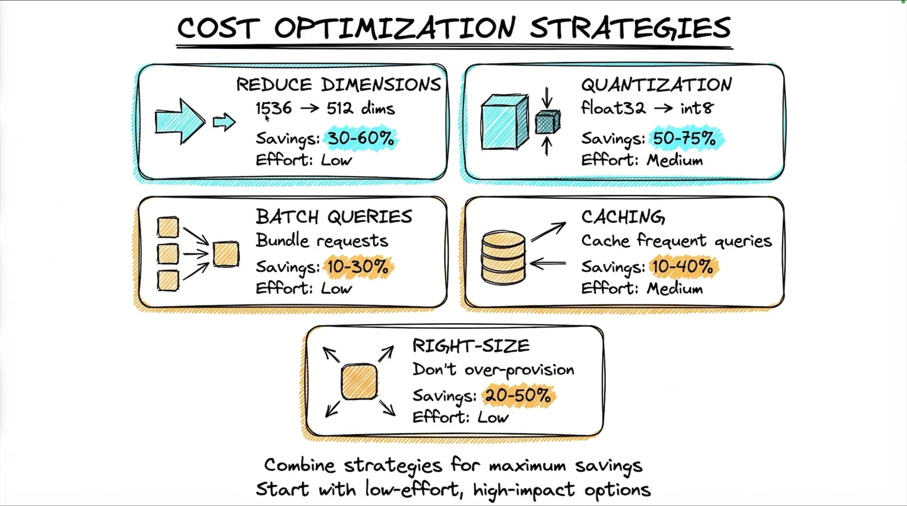
| # | Strategy | Savings | Effort | Ratio verdict |
|---|---|---|---|---|
| 1 | Reduce dimensions (1536 → 512) | 30–60% | Low | Do this first |
| 5 | Right-size (don't over-provision) | 20–50% | Low | Do this second, forever |
| 3 | Batch queries (bundle requests) | 10–30% | Low | Do this third |
| 2 | Quantization (float32 → int8) | 50–75% | Medium | Biggest saver, real work |
| 4 | Caching (cache frequent queries) | 10–40% | Medium | Depends entirely on your repeat rate |
The slide's instruction: "Combine strategies for maximum savings. Start with low-effort, high-impact options."
Lever 1 — reduce dimensions (1536 → 512)
Storage, index size, RAM footprint and per-query distance computation all scale linearly with the number of floats per vector. Most teams are on OpenAI's default 1536 dimensions and never touch the setting. Dropping to 512 is a 3× reduction in vector payload for 30–60% savings at Low effort — the best ratio on the board.
"So that's one thing people don't talk about." 03:28:12
With the raw OpenAI SDK it is one keyword argument:
# Slide only, [03:28:35] — this exact snippet is NOT in either course repo.
response = client.embeddings.create(
    model='text-embedding-3-small',
    input='Your text',
    dimensions=512  # Reduced from 1536
)
And it is sticky: everything produced through that instantiated model comes out at 512 dimensions from then on 03:28:38. The LangChain equivalent is a constructor argument — OpenAIEmbeddings(model="text-embedding-3-small", dimensions=512) — and it is only honoured by text-embedding-3 and later models, so text-embedding-ada-002 cannot be shrunk this way. The repo's embeddings_deep.py line 8 is the "before" picture: OpenAIEmbeddings(model="text-embedding-3-small") with no dimensions argument, i.e. the 1536-d default.
Be precise about which meter this moves. Embedding APIs bill on input tokens, not on output floats, so asking for 512 dimensions instead of 1536 does not make the embedding call cheaper by one cent. What it shrinks is the storage row, the index's RAM footprint and the per-query distance computation — rows 2 and 3 of the table at the top of this part. That is why the savings band is quoted against infrastructure cost and why the lever pays off more the larger your corpus gets.
The cost half of the trade-off is what chapter 16 gives you. The quality half was established back in Part 4: fewer dimensions means less semantic nuance, with the sweet spot for most use cases at 768–1536. 512 sits below that band. Chapter 16 asserts the savings and never measures the recall delta, so treat "reduce to 512" as a hypothesis to A/B on your own corpus with your own retrieval test (Part 3's methodology: measure end-to-end retrieval, never eyeball the vectors).
Lever 2 — quantization (float32 → int8)
Where dimension reduction cuts the number of dimensions, quantization cuts the bytes per dimension 03:28:47. float32 → int8 is 4 bytes → 1 byte, a 4× reduction; binary quantization goes further. Rated 50–75% savings, Medium effort.
The two levers are orthogonal and they compose: 1536→512 is 3×, float32→int8 is 4×, and stacked they are roughly 12× smaller vectors. (The instructor never performs that multiplication; the slide's "combine strategies" line is the same claim in prose. The arithmetic is this guide's, and it is an upper bound on storage, not a promise about recall.)
Lever 3 — batch queries
The anti-pattern is the default coding habit — a for loop over queries — which is what makes it dangerous:
"if you have 10,000 API calls doing this that's crazy. That's a lot." 03:29:42
# Slide only, [03:29:52] — generic vector-DB SDK, illustrative.
# Bad: 10,000 API calls
for query in queries:
    results = index.query(query)

# Good: Batched queries (if supported)
results = index.query(queries, batch=True)
The for-loop is not wrong logic, it is wrong economics under per-request pricing. The mechanism is stated exactly once and it is the whole model:
"fewer round trips, which means lower costs on usage-based pricing. That's the key." 03:29:59
10–30% savings, and the effort is described as "extremely low" 03:29:14.
And do not mistake LangChain's .batch() for this. Every Runnable — retrievers included — exposes .batch([...]), and its default implementation runs invoke once per input across a thread pool: N concurrent calls, not one call. Its own docstring says so, and adds that subclasses "must override this method if they can batch more efficiently." So .batch() cuts wall-clock latency and cuts nothing off a usage-based bill unless the specific integration overrode it. Server-side batching is a property of the vendor's API, not of the orchestration layer — check per component, never assume.
You are, however, probably already batching on the index side without noticing. embeddings_model.embed_documents([...]) takes a list and packs it into requests of up to chunk_size pieces each (LangChain's default for OpenAIEmbeddings is 1000) — that is a genuine server-side batch, and it is why bulk ingestion is cheap. embed_query(text) takes a single string and is what you pay one request for on every question. The asymmetry is structural: the index path is batchable by construction, the query path is not, because the query does not exist until the user types it. Where you can genuinely batch on the read path is offline work — evaluation runs, nightly re-scoring, backfills.
Lever 4 — caching, quantified in one sentence
"if 20% of queries are repeats, you save 20% on compute" 03:30:13
The savings percentage is the repeat rate. That is the entire economic model, and it means the decision to build a cache is empirical: measure your repeat rate first. Slide range: 10–40% savings, Medium effort.
The canonical scenario is a support bot 03:30:20 — support and FAQ traffic has a heavy head where a handful of questions dominate volume, which is exactly the distribution an LRU cache rewards. A research tool over a unique-document corpus has the opposite distribution and a cache there is dead weight.
Two things can be cached, at two different layers 03:30:32:
- the retrieval result — skip hitting the vector database
- the response — skip the LLM call as well
Caching gets its own full section below, because chapter 18 builds both layers properly.
Lever 5 — right-size, the one nobody does
20–50% savings at Low effort — and it is the strategy people skip, because it never finishes. The loop 03:31:24:
- Start with a small instance.
- Monitor usage.
- Scale only when you hit actual limits — not on projection.
- Review costs monthly.
- Repeat forever.
"This is the thing, okay? It's a process." 03:31:39
A one-time right-size drifts out of date the moment your traffic shape changes 03:31:53. This is the lever that most directly depends on Part 7: without usage metrics, step 2 is guesswork and step 3 is superstition.
Caching, properly: three layers, three implementations
Chapter 18 changes subject at 03:54:27 from Supabase (Part 10) to caching, and builds two of the three layers in real code. Combined with chapter 16's retrieval cache, you get the full stack.
| Layer | What it skips | Key | Typical hit rate | Where taught |
|---|---|---|---|---|
| Embedding cache | the embedding API call | chunk text (hashed) | ~100% on an unchanged re-ingest | ch18 03:54:27 |
| Retrieval cache | the vector search | query (MD5) | = repeat rate | ch16 03:30:32 |
| Response cache | the whole LLM call | normalised query (MD5) | 30–50% | ch18 03:58:32 |
They compose. A cached response short-circuits everything behind it; a cached retrieval still pays for generation; a cached embedding only saves the embedding call. Order the checks outermost-first.
Layer 1 — the embedding cache
"Caching is very important especially when it comes to embeddings because it avoids redundant API calls." 03:54:27
The logic is unarguable: embedding is an inference call, it is billed on tokens (Part 4), and identical text always produces an identical vector. Embedding the same text twice is pure waste. It pays off whenever the same chunk text passes the embedder twice: re-running an ingest that crashed halfway, rebuilding an index into a new store, re-ingesting a corpus where only a few documents changed, or the demo-in-a-loop habit from Part 4 where every run re-embeds everything.
Know its limit, though, because it is easy to overestimate. The key is derived from the text, so changing your chunker invalidates the entire cache — different boundaries mean different strings mean different keys. The one re-index you most want to be free is exactly the one that isn't.
LangChain's answer is a decorator around any embeddings model, backed by any byte store:
# production-course-main-code/embeddings_deep.py — lines 69-97
def embedding_caching():
    from langchain_classic.embeddings.cache import CacheBackedEmbeddings

    from langchain_classic.storage import LocalFileStore
    import tempfile

    with tempfile.TemporaryDirectory() as tempdir:
        store = LocalFileStore(root_path=tempdir)

        cached_embeddings = CacheBackedEmbeddings.from_bytes_store(
            underlying_embeddings=embeddings_model,
            document_embedding_cache=store,
            namespace="exercise",
        )

        text = "What is Reinforcement Learning?"

        # First call - hits API
        print("First call (API):")
        vectors1 = cached_embeddings.embed_documents([text])
        print(f"  Embedded {len(vectors1)} documents")

        # Second call - from cache
        print("\nSecond call (Cache):")
        vectors2 = cached_embeddings.embed_documents([text])
        print(f"  Embedded {len(vectors2)} documents")

        # Verify same results
        print(f"\nSame vectors: {np.allclose(vectors1[0], vectors2[0])}")
Run it with uv run embeddings_deep.py and the last line prints Same vectors: True 03:58:32. Note the verification method: compare the vectors, not the timings. Timing is noisy and machine-dependent; vector equality is a proof. Note also what the demo does not prove — both calls report Embedded 1 documents, so the printed counts are identical whether or not the cache fired. Only np.allclose tells you anything.
The store interface is deliberately minimal — per the on-screen docstring, it "works with any store that implements the abstract store interface accepting keys of type str and values of list of floats" 03:58:20. LocalFileStore is one implementation of that ByteStore; a Redis-, S3- or database-backed store drops in unchanged, which is what makes this pattern shareable across workers.
namespace is not decoration. 03:56:30 The cache key is derived from the text, not the model. Cache text-embedding-3-small and text-embedding-3-large vectors for the same string without namespacing and you will serve a 3072-d vector to a 1536-d index — invariant 2 violated silently, by your own cache. LangChain's own docstring says to set it to the name of the embedding model used; because dimensions are part of the model's identity, namespace by model and by dimensions. The demo's namespace="exercise" is a teaching name, not a pattern to copy.
One more default worth knowing before you count your savings: from_bytes_store takes query_embedding_cache, and it is False. Out of the box this caches document embeddings only — the per-request embed_query call, the one on your hot path, is not cached at all. Pass query_embedding_cache=True to reuse the same store for queries, which is what actually pays off when the same question arrives twice.
The SHA-1 warning is worth reading rather than dismissing. It is raised by _warn_about_sha1_encoder() and reported at its call site, langchain_classic/embeddings/cache.py:58. It says, in substance: SHA-1 is not collision-resistant, a motivated attacker can craft two different payloads that map to the same cache key, supply a stronger encoder via the key_encoder argument — and if you change the encoder, create a new cache to avoid collisions with existing keys. key_encoder accepts a callable or one of the literals "sha1", "blake2b", "sha256", "sha512".
The instructor's advice is:
"You got to get that warning, but you can just ignore all of that." 03:58:32
That is fine for a local single-user demo and wrong for a shared or multi-tenant cache, where a crafted collision means one tenant is served another tenant's vector. Pass key_encoder="sha256" and move on; it costs nothing.
Layer 2 — the retrieval cache
Chapter 16 shows this one on a slide, gets it wrong, catches itself on air, and fixes it — which makes it a better teaching artefact than a clean version would have been.
"I notice that I have a little bug here." 03:31:11
# Slide v1, [03:31:20] — BROKEN, shown here as the trap.
import hashlib
from functools import lru_cache

@lru_cache(maxsize=1000)
def cached_search(query_hash):          # `query` is not in scope
    return vectorstore.similarity_search(query)

def search(query):
    query_hash = hashlib.md5(query.encode()).hexdigest()
    return cached_search(query_hash)
# Slide v2, [03:31:24] — the corrected version.
import hashlib
from functools import lru_cache

@lru_cache(maxsize=1000)
def cached_search(query_hash, query):
    return vectorstore.similarity_search(query)

def search(query):
    query_hash = hashlib.md5(query.encode()).hexdigest()
    return cached_search(query_hash, query)
The v1 body references query, which is never a parameter. At best that is a NameError; at worst it silently closes over a module-level query and returns results for the wrong question — a cache that answers confidently and incorrectly, which is the worst possible failure in a RAG system.
Two things the corrected version buys you for free. functools.lru_cache(maxsize=1000) provides bounded, least-recently-used eviction with zero infrastructure — no Redis, no service, six lines 03:31:20. And MD5 is used purely as a fixed-length content fingerprint 03:31:02, which keeps the key uniform regardless of query length. It is not a security primitive here and must never be repurposed as one.
Layer 3 — the response cache
The thesis is one sentence 03:58:32:
"Don't pay twice for the same answer."
Two steps per lookup — normalise, then hash. (The instructor calls this a "two-layer cache." He means the two steps above, not two of the three cache layers in the table. Same word, different axis; do not let it confuse you.)
# production-course-main-code/cost_optimization.py — lines 101-133
class SemanticCache:
    """Cache responses with semantic similarity matching."""

    def __init__(self, similarity_threshold: float = 0.9):
        self.cache = {}
        self.threshold = similarity_threshold
        self.embedder = ChatOpenAI(model="gpt-4o-mini", temperature=0)

    def _hash_query(self, query: str) -> str:
        """Create hash of normalized query."""
        normalized = query.lower().strip()
        return hashlib.md5(normalized.encode()).hexdigest()

    def get(self, query: str) -> Optional[str]:
        """Get cached response if similar query exists."""
        query_hash = self._hash_query(query)

        # Exact match
        if query_hash in self.cache:
            return self.cache[query_hash]["response"]

        # Could add embedding-based similarity here
        # For demo, just use exact match

        return None

    def set(self, query: str, response: str):
        """Cache a response."""
        query_hash = self._hash_query(query)
        self.cache[query_hash] = {"query": query, "response": response}

    def stats(self) -> dict:
        return {"cached_queries": len(self.cache)}
Step 1 is query.lower().strip() 03:58:32 — cheap wins, because users type the same question in different cases and with stray whitespace. Step 2 is MD5 into a fixed-length hex digest 03:59:33, "really fast as well."
The wrapper adds the counters and the tracing:
# production-course-main-code/cost_optimization.py — lines 145-174
    @traceable(name="cached_invoke")
    def invoke(self, query: str) -> tuple[str, bool]:
        """
        Invoke with caching.
        Returns: (response, from_cache)
        """
        # Check cache
        cached = self.cache.get(query)
        if cached:
            self.cache_hits += 1
            return cached, True

        # Call LLM
        self.cache_misses += 1
        response = self.llm.invoke(query)
        result = response.content

        # Cache result
        self.cache.set(query, result)

        return result, False

    def get_stats(self) -> dict:
        total = self.cache_hits + self.cache_misses
        hit_rate = self.cache_hits / total if total > 0 else 0
        return {
            "hits": self.cache_hits,
            "misses": self.cache_misses,
            "hit_rate": f"{hit_rate:.1%}",
        }
Three design details worth stealing. invoke returns a tuple (result, from_cache: bool) 04:00:34 so the caller can tell where the answer came from — which is what makes the demo print [CACHE] vs [LLM], and what lets a real API attach a X-Cache: HIT header or a cache_hit=True metric. The cached path is still traced (@traceable(name="cached_invoke")) 04:00:34 — caching and observability are not alternatives; you want the hits in your traces precisely so you can compute the hit rate from the same source of truth as everything else. And on a hit the answer returns "instantly. So it's free. There's no latency essentially." 04:01:37 — this is a latency optimisation dressed as a cost optimisation.
The demo, and the number it produces
# production-course-main-code/cost_optimization.py — lines 177-197
def demo_caching():
    """Demonstrate caching."""

    llm = CachedLLM()

    queries = [
        "What is Python?",
        "What is JavaScript?",
        "What is Python?",  # Cache hit
        "What is python?",  # Cache hit (normalized)
        "What is Rust?",
    ]

    print("\nCaching Demo:\n")

    for query in queries:
        result, from_cache = llm.invoke(query)
        source = "CACHE" if from_cache else "LLM"
        print(f"[{source}] {query} -> {result[:30]}...")

    print(f"\nStats: {llm.get_stats()}")
Five queries, and the fourth is the interesting one: "What is python?" hits only because of the .lower() in _hash_query. The printed result 04:03:00:
Stats: {'hits': 2, 'misses': 3, 'hit_rate': '40.0%'}"40% hit rate means 40% of your LLM calls were eliminated. Two of our five queries cost zero." 04:02:40
⚠️ To reproduce this you must edit the file. The shipped __main__ block has demo_caching() commented out and runs demo_token_budgeting() instead. Uncomment it, then uv run cost_optimization.py — the command used on screen.
Provenance note. On screen at recording time the file ended right after demo_caching() — the "Production version would…" comment sat at lines 205–208, not 294–297. The entire # === Token Budgeting === section (TokenBudget, BudgetedLLM, demo_token_budgeting) was appended to the repo after this chapter was recorded, which is why the two halves of this part come from chapters an hour and a half apart yet live in one file. ModelRouter was already there and simply not discussed. The caching demo was also recorded in a different workspace (langc-course, Python 3.12.2) from the Supabase half of the same chapter.
Expect 30–50% hit rates in production 04:02:40, because real traffic is repetitive — the instructor's examples are "How do I reset my password?" and "What are your business hours?". That saves money and latency: "the users get the response right away."
What this cache is not
The class is called SemanticCache and it is not semantic. The instructor says so himself 04:02:40: after normalisation it is still a string equality test. "What is Python" and "Tell me about Python" mean the same thing and hash differently, so they miss.
The file carries four further artefacts that will confuse anyone extending it:
self.embedder = ChatOpenAI(model="gpt-4o-mini", temperature=0)— a chat model assigned to
a variable named embedder, and never used. A real implementation needs OpenAIEmbeddings. This is the single most misleading line in the chapter.
similarity_threshold(default0.9) is stored and never read. No code path consumes
self.threshold 03:59:33.
if cached:conflates "missing" with "empty".SemanticCache.get()returnsNoneon a miss,
but the wrapper tests truthiness, so a cached empty-string answer is treated as a miss and re-billed on every request forever. Test is not None.
self.cache = {}is unbounded and per-process. It never evicts (a long-running server leaks),
and behind N workers your effective hit rate is divided by N. lru_cache(maxsize=1000) from layer 2 solves the first problem; only a shared backing store solves the second — either your own Redis, or LangChain's global cache hook, langchain_core.globals.set_llm_cache(...), pointed at a shared backend.
The instructor's defence is that the naming is aspirational on purpose:
"It's built to be extended with embeddings. So the exact match version is the starting point." 04:03:41
The upgrade to a real semantic cache
The recipe is a trailing comment in the file, and it is the last thing chapter 18 says before it runs out of tape:
# production-course-main-code/cost_optimization.py — lines 294-297
    # Production version would:
# 1. Embed the query into a vector
# 2. Search the cache by vector similarity
# 3. Return if similarity > threshold (e.g., 0.95)
Three steps, all of which you already know how to build from Parts 4 through 6: embed the query, search a small vector store of cached questions, return the stored answer if the top similarity clears the threshold.
Measure before you build
monitoring.py already gives you the instrument:
# production-course-main-code/monitoring.py — lines 106-111
        cache_hit_rate = (
            self.metrics["cache_hits"]
            / (self.metrics["cache_hits"] + self.metrics["cache_misses"])
            if (self.metrics["cache_hits"] + self.metrics["cache_misses"]) > 0
            else 0
        )
MetricsCollector.get_summary() folds that into a cache_hit_rate string alongside error rate and average latency, so the number lands in the same summary as everything else.
Run a no-op cache first — hash every query, record hit or miss, always call the LLM. After a week you know your real repeat rate, and therefore, per chapter 16's model, you know your exact savings before you have written a line of caching logic. The same instrument answers the right-sizing question in the next section; that is not a coincidence, it is why Part 7 comes before this part.
Which vector database, by corpus scale
Chapter 16 lands on a lookup table indexed by one number: how many vectors you have.
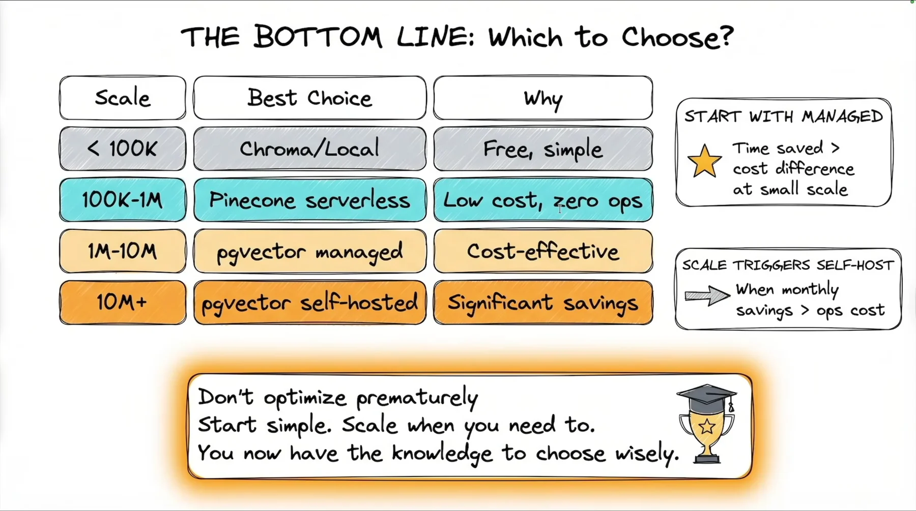
| Scale | Best choice | Why |
|---|---|---|
| < 100K | Chroma / local | Free, simple — and, as Part 4 showed, quick 03:32:10 |
| 100K – 1M | Pinecone serverless | Low cost, zero ops |
| 1M – 10M | pgvector managed | Cost-effective |
| 10M+ | pgvector self-hosted | Significant savings |
And the two side rules that actually govern the decision:
- START WITH MANAGED — "Time saved > cost difference at small scale." 03:32:40 At the
bottom of the curve the dollar gap is smaller than the value of the engineering hours you would burn running your own Postgres.
- SCALE TRIGGERS SELF-HOST — "When monthly savings > ops cost." This box appears on the slide
only; the instructor never reads it aloud, which makes it easy to miss and it is the most important sentence on the page.
The closing instruction is the one that saves the most money in practice:
"Don't optimize prematurely. Start simple. Scale when you need to." (slide, 03:32:05)
The spoken version adds the payoff, and it is the correct reading of this whole part: the point of learning to self-host is not to self-host now — it is that "when you hit scale, where costs matter, you will have the knowledge from this course to self-host effectively" 03:32:58. The chapter signs off as the end of the vector-database-to-production arc 03:33:08.
Two cross-references so you can act on this table. The index tuning that decides whether you need the next tier at all — HNSW M and ef, vertical vs horizontal scaling — is Part 8. The concrete hosting SKUs behind the "pgvector managed" row — Supabase, Neon, AWS RDS, with real monthly prices — are Part 10.
The latency budget
Money gets a whole chapter; latency gets scattered sentences. Assemble them yourself, because your users feel latency and only your CFO feels cost.
Across the three chapters behind this part, the source gives exactly one hard latency number: hybrid search adds ~20–50 ms, because you are literally running two retrievals instead of one 02:12:09. Everything else is qualitative, so the table below mixes sourced figures with explicitly-marked derivations. Do not treat any unmarked row as measured — measure it yourself:
| Stage | Latency contribution | Source |
|---|---|---|
| Token-budget gate | ~0 (a .split() and a comparison) | derived |
| Response-cache hit | ~0 — "it's free. There's no latency essentially" | 04:01:37 |
| Query embedding | one API round trip | not quantified in source |
| Vector search | grows with index size and ef | Part 8 |
| + BM25 branch (hybrid) | +20–50 ms | 02:12:09 |
| + Reranking | one model pass over k candidates | Part 6 |
| + Routing classifier | one full extra LLM round trip | 02:20:25 |
| LLM generation | dominant; grows with input and output tokens | derived |
Three rules fall out of that table.
Order the pipeline cheapest-first. The production request pipeline from Part 1 — Client → Rate limiter → Security → Cache → Model (+retry +fallback) → Output validation → Metrics → Response — is a latency and cost ordering as much as a security one. Cheap rejections first, expensive inference last. A token-budget gate placed after the retrieval call has already spent your money and your milliseconds.
Some cost optimisations are latency pessimisations. Model routing saves money and adds a full LLM round trip to every request 02:20:25. Hybrid search buys accuracy and spends 20–50 ms. Summary memory bounds token cost and adds an extra LLM call at every overflow. There is no free lunch here — this is invariant 5, every layer is a "pick 2", expressed in milliseconds.
Some are both. Caching is the one unambiguous win: a hit costs zero dollars and zero milliseconds. This is why caching, despite its Medium effort rating and its unremarkable 10–40% savings band, is usually the first thing to build after right-sizing.
And the Pods row from the pricing table earlier is the only line item in this entire part that is purely a latency purchase: 2–5× the Serverless price, buying nothing but a tail-latency guarantee 03:24:14. If you have a p99 SLA, that premium is not waste; if you do not, it is.
Putting a number on it: a worked cost model
The course never multiplies its own constants together. Doing so is the fastest way to see which lever matters. The arithmetic below is derived, not quoted — but every constant in it is a documented figure, and each carries its source.
The workload is chapter 16's baseline 03:24:02: 500K vectors, 10,000 queries/day. The request shape is the one the course models in its own long-context-vs-RAG calculator (Part 14): 4 retrieved chunks × 500 tokens of context, a 100-token query, a 500-token answer — 2,100 tokens in, 500 out. The prices are text-embedding-3-small at $0.02/1M tokens (Part 4), gpt-4o-mini input at $0.15/1M ($0.00015/1K, hardcoded in cost_optimization.py), and gpt-4o at $2.50/1M input, $10.00/1M output (the constants in the course's calculator).
Index-time, one-time. 500K chunks × 500 tokens = 250M tokens → $5.00 to embed the entire corpus. Once. This is invariant 3 made concrete: the number everyone worries about is the cheapest number on the page — until you change your chunker, at which point you pay it again.
Query-time embedding. 100 tokens × 10,000/day × 30 = 30M tokens/month ≈ $0.60/month. Negligible — which is precisely why dimension choice is a storage-and-latency decision, not an embedding-bill decision.
Vector database. Chapter 16's baseline: $20–30/month on Pinecone Serverless, $15–20 self-hosted.
Generation, per request, 2,100 in + 500 out:
- On
gpt-4o: 2,100 × $2.50/1M = $0.00525 in, plus 500 × $10.00/1M = $0.00500 out →
$0.01025 per request. At 10,000 queries/day that is $102.50/day — the exact figure 01_long_context_vs_rag.py prints in its own "at 10,000 queries/day" block → ~$3,075/month.
- On
gpt-4o-mini: the repo prices input only — 2,100 × $0.15/1M = $0.000315 per request →
~$95/month, and that is a floor. The mini output rate appears nowhere in the source.
Read the first bullet again: at this shape the output tokens cost as much as the input tokens, even though the input is four times larger, because output is priced 4× higher per token. Any cost model that prices only the input — and the course's own ModelRouter does exactly that — is out by roughly a factor of two.
| Meter | Monthly at 500K / 10K queries per day | Share |
|---|---|---|
| Corpus embedding ($5.00 once, amortised over a year) | ~$0.42 | <1% |
| Query embedding | ~$0.60 | <1% |
| Vector DB (Pinecone Serverless) | $20–30 | ~24% |
Generation (gpt-4o-mini, input only) | ~$95 | ~75% |
Shares are computed at the $30 top of the vector-DB range; at $20 the generation share rises to 82%. On gpt-4o the comparison stops being a comparison: ~$3,075 of generation against $20–30 of database is a 1% infrastructure bill.
Three caveats, stated rather than buried. (1) This assumes one LLM call per query — multi-query, reranking, a routing classifier or an agent loop each multiply the generation row and none of them touch the database row. (2) Prices are the ones in the repo and slides at recording time and will drift; keep your own price table and version it. (3) The database row is the one that goes superlinear: at 50M vectors it is $1,500+/month while the generation row per request has not moved. The ranking in this table is a function of your scale, so re-run it at 10× before acting.
Now apply the levers. A 40% response-cache hit rate removes 40% of both the generation and query-embedding rows: ~$95 → ~$57 on mini, ~$3,075 → ~$1,845 on gpt-4o. It is the only lever that touches the biggest row. Routing half your traffic from gpt-4o to gpt-4o-mini takes the input half of the bill from ~$1,575 to ~$835, minus the classifier's own per-request cost. Dimension reduction touches none of these rows except the $20–30 one — and it is still worth doing, because that is the row that becomes $1,500+ at 50M vectors.
Decisions to make
Work top to bottom. Each item is a decision with a default, not a task.
- What is your workload, in two numbers? Vector count and queries/day. Write them down. Every
price in this part is meaningless without both. Re-price at 10× and 100× your current numbers before you pick a vendor — the ranking inverts.
- Which vector DB tier? <100K → Chroma/local. 100K–1M → Pinecone serverless. 1M–10M → pgvector
managed. 10M+ → pgvector self-hosted. Default to managed while small, and migrate on the inequality monthly savings > ops cost, not on hitting a vector count.
- What is your embedding dimension, and did you choose it? 1536 is a default, not a decision.
512 saves 30–60% at Low effort but costs semantic nuance and cannot be changed without a full re-embed. Decide before your first production ingest. A/B recall on your own corpus.
- Is there a pre-flight token gate on every user-facing endpoint?
TokenBudgetwith a
max_tokens_per_request you have actually justified (the code's default is 4,000). The check must run before the API call. Add a second, independent cap on output tokens, and replace .split() with a character-length guard too, or a space-free payload walks straight through.
- Are your token counters dimensioned by user, hour and endpoint? If you cannot answer "who is
driving my cost", you cannot rate-limit, bill or negotiate. Bill from AIMessage.usage_metadata, never from a words × 1.3 estimate; keep the estimate for the gate, where no response exists yet.
- Do you know your query repeat rate? Instrument a no-op cache for a week before building a
real one. Savings ≈ repeat rate. Expect 30–50% on support/FAQ traffic and near zero on research-style traffic.
- Which cache layers are you running? Embedding cache (persistent store, namespaced by model
and dimensions, key_encoder="sha256", query_embedding_cache=True if you want query-side savings), retrieval cache (lru_cache(maxsize=1000), normalised key, return a copy), response cache (normalise → hash → bounded store). Never a bare unbounded dict in a multi-worker server — use a shared backend, via your own Redis or langchain_core.globals.set_llm_cache.
- Is your "semantic" cache actually semantic? If it is the course's
SemanticCache, it is
exact-match after .lower().strip() — rename it honestly, or implement the upgrade: embed → vector search → return above a threshold. Start at the source's higher figure (0.95, not the constructor's 0.9), log every hit's similarity score, and tune down only on evidence.
- Have you capped conversation growth? Pick one of trim / window / summarise and know what each
destroys. Trimming and windowing lose old facts silently; summarising preserves them, costs an extra LLM call per overflow, and drifts. Log the summary either way.
- Is model routing paying for itself, and which way does it fail? The classifier is a full LLM
call per request. Compare classifier spend against routed savings monthly, try a heuristic classifier first, and make the cheap model the fallback for any unrecognised classification — the course's version does the opposite.
- Are you batching where the SDK supports it? Confirm support before designing around it.
embed_documents([...]) is already a server-side batch; a Runnable's .batch() is only client-side concurrency; index.query(queries, batch=True) may or may not exist in your client.
- When is your monthly cost review? Right-sizing is 20–50% at Low effort and it is the lever
people skip because it never ends. Small instance → monitor → scale on real limits → review monthly → repeat.
- Have you written down the latency budget? One row per stage, a p95 allowance in each, then a
timer on each row (Part 7). Ship the table before you optimise anything — hybrid costs 20–50 ms, routing costs a full round trip, a cache hit costs nothing, and the row that is lying to you is never the one you suspect.
- Have you re-run this whole list at 10× your current scale? Every ranking in this part is a
function of workload: the vector DB is ~24% of the bill at 500K vectors and the dominant line at 50M, while the per-request generation cost does not move. Put the re-run on the same calendar entry as the monthly cost review.